←Back to CS 180
P3

Project 3: (Auto)Stitching Photo Mosaics

October 17, 2025

Image WarpingImage Mosaicing

Overview

The goal of this assignment is to play with image warping and mosaicing. Take two or more photographs and create an image mosaic by registering, projective warping, resampling, and composing them. Along the way, learn how to compute homographies, and how to use them to warp images.

Image Warping and Mosaicing

A.1: Shoot the Pictures

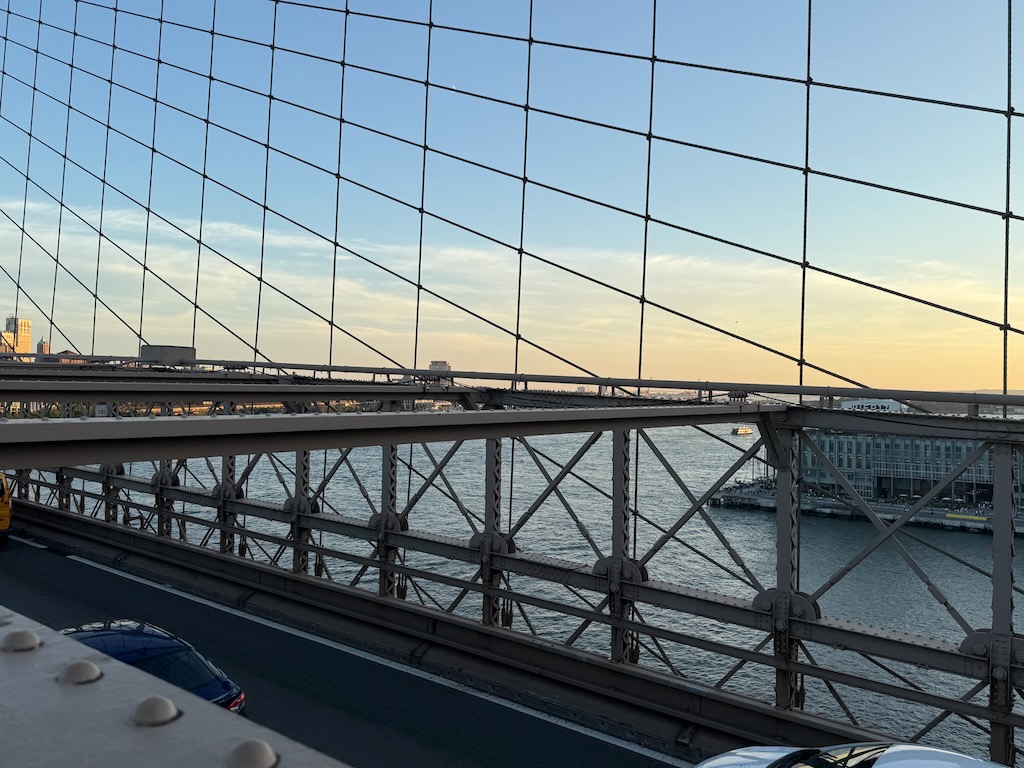
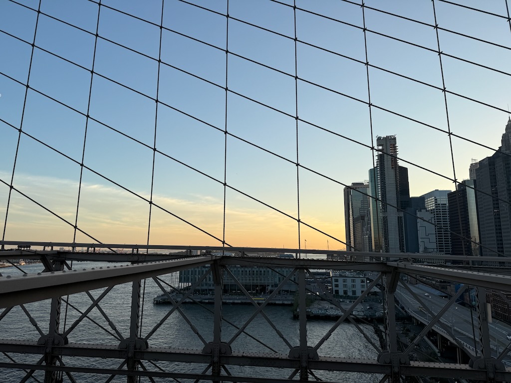
Shoot two or more photographs so that the transforms between them are projective (a.k.a. perspective). The most common way is to fix the center of projection (COP) and rotate your camera while capturing photos.

Brooklyn Bridge at Sunset...

Brooklyn Bridge at Sunset...

with a slightly different angle

with a slightly different angle

A.2: Recover Homographies

We define a single correspondence (x,y,1)↦λ(u,v,1)(x, y, 1) \mapsto \lambda (u, v, 1) (homogeneous coordinates) by the projective transformation matrix

H=[h1h2h3h4h5h6h7h8h9] H = \begin{bmatrix} h_{1} & h_{2} & h_{3}\\ h_{4} & h_{5} & h_{6}\\ h_{7} & h_{8} & h_{9} \end{bmatrix}
with
λ[uv1]=H[xy1] \lambda \begin{bmatrix} u\\ v\\ 1\end{bmatrix} = H \begin{bmatrix} x\\ y\\ 1\end{bmatrix}
Write the scalar equations:
λu=h1x+h2y+h3,λv=h4x+h5y+h6,λ=h7x+h8y+h9. \begin{aligned} \lambda u &= h_{1}x + h_{2}y + h_{3},\\\\ \lambda v &= h_{4}x + h_{5}y + h_{6},\\\\ \lambda &= h_{7}x + h_{8}y + h_{9}. \end{aligned}
Eliminate λ\lambda using the third equation:
u (h7x+h8y+h9)=h1x+h2y+h3,v (h7x+h8y+h9)=h4x+h5y+h6. \begin{aligned} u\,(h_{7}x + h_{8}y + h_{9}) &= h_{1}x + h_{2}y + h_{3},\\\\ v\,(h_{7}x + h_{8}y + h_{9}) &= h_{4}x + h_{5}y + h_{6}. \end{aligned}
Bring all terms to the left-hand side:
xh1+yh2+h3−uxh7−uyh8−uh9=0,xh4+yh5+h6−vxh7−vyh8−vh9=0. \begin{aligned} x h_{1} + y h_{2} + h_{3} - u x h_{7} - u y h_{8} - u h_{9} &= 0,\\\\ x h_{4} + y h_{5} + h_{6} - v x h_{7} - v y h_{8} - v h_{9} &= 0. \end{aligned}
Assume h9=1h_{9} = 1 (fixing scale) and move constants to the right:
xh1+yh2+h3−uxh7−uyh8=u,xh4+yh5+h6−vxh7−vyh8=v. \begin{aligned} x h_{1} + y h_{2} + h_{3} - u x h_{7} - u y h_{8} &= u,\\\\ x h_{4} + y h_{5} + h_{6} - v x h_{7} - v y h_{8} &= v. \end{aligned}
Flatten the unknowns into vector form:
h=[h1h2h3h4h5h6h7h8]. \mathbf{h} = \begin{bmatrix} h_{1}\\ h_{2}\\ h_{3}\\ h_{4}\\ h_{5}\\ h_{6}\\ h_{7}\\ h_{8} \end{bmatrix}.
For a single correspondence (x,y)↦(u,v)(x, y) \mapsto (u, v), we get two equations:
[ x    y    1    0    0    0    −ux    −uy ]h=u,[ 0    0    0    x    y    1    −vx    −vy ]h=v. \begin{aligned} [\,x \;\; y \;\; 1 \;\; 0 \;\; 0 \;\; 0 \;\; -u x \;\; -u y\,] \mathbf{h} &= u,\\\\ [\,0 \;\; 0 \;\; 0 \;\; x \;\; y \;\; 1 \;\; -v x \;\; -v y\,] \mathbf{h} &= v. \end{aligned}
Thus, to solve for h1,...,h8h_{1},...,h_{8} (8 unknowns) we need 4 correspondences. Stacking them gives:
[x1y11000−u1x1−u1y1000x1y11−v1x1−v1y1x2y21000−u2x2−u2y2000x2y21−v2x2−v2y2x3y31000−u3x3−u3y3000x3y31−v3x3−v3y3x4y41000−u4x4−u4y4000x4y41−v4x4−v4y4]⏟A[h1h2h3h4h5h6h7h8]=[u1v1u2v2u3v3u4v4]. \underbrace{\begin{bmatrix} x_1 & y_1 & 1 & 0 & 0 & 0 & -u_1 x_1 & -u_1 y_1\\ 0 & 0 & 0 & x_1 & y_1 & 1 & -v_1 x_1 & -v_1 y_1\\ x_2 & y_2 & 1 & 0 & 0 & 0 & -u_2 x_2 & -u_2 y_2\\ 0 & 0 & 0 & x_2 & y_2 & 1 & -v_2 x_2 & -v_2 y_2\\ x_3 & y_3 & 1 & 0 & 0 & 0 & -u_3 x_3 & -u_3 y_3\\ 0 & 0 & 0 & x_3 & y_3 & 1 & -v_3 x_3 & -v_3 y_3\\ x_4 & y_4 & 1 & 0 & 0 & 0 & -u_4 x_4 & -u_4 y_4\\ 0 & 0 & 0 & x_4 & y_4 & 1 & -v_4 x_4 & -v_4 y_4 \end{bmatrix}}_{\mathbf{A}} \begin{bmatrix} h_1\\ h_2\\ h_3\\ h_4\\ h_5\\ h_6\\ h_7\\ h_8 \end{bmatrix} = \begin{bmatrix} u_1\\ v_1\\ u_2\\ v_2\\ u_3\\ v_3\\ u_4\\ v_4 \end{bmatrix}.
Finally, solve the system for h\mathbf{h} to reconstruct the homography:
H=[h1h2h3h4h5h6h7h81]. H = \begin{bmatrix} h_1 & h_2 & h_3\\\\ h_4 & h_5 & h_6\\\\ h_7 & h_8 & 1 \end{bmatrix}.
* While 4 correspondences is the minimum necessary to solve for 8 unknowns of HH, having more correspondences makes the final projection transformation matrix more robust to noise in correspondence choices because we can solve the overdetermined system using least squares.

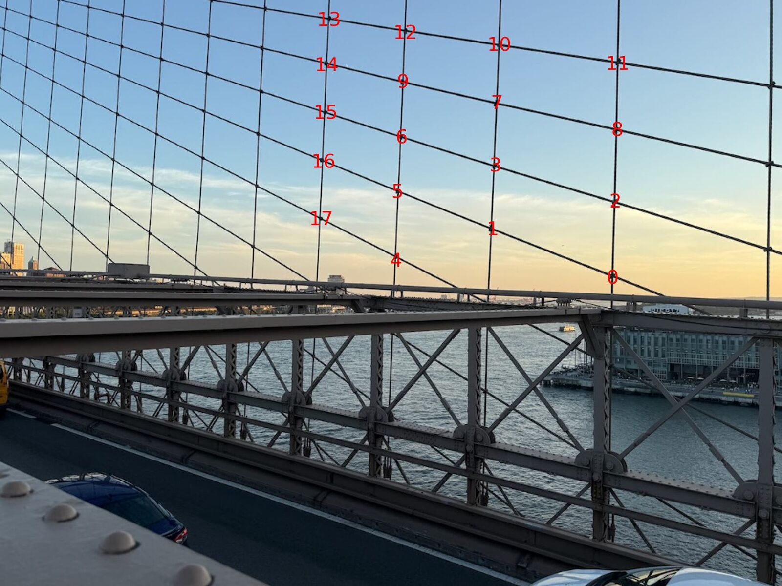
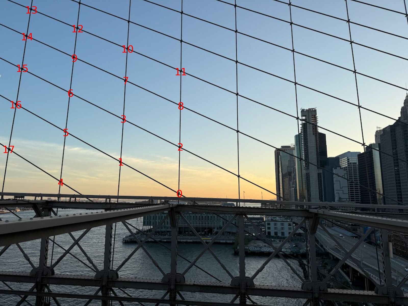
Point Correspondences

Point...

Correspondencse

Correspondences

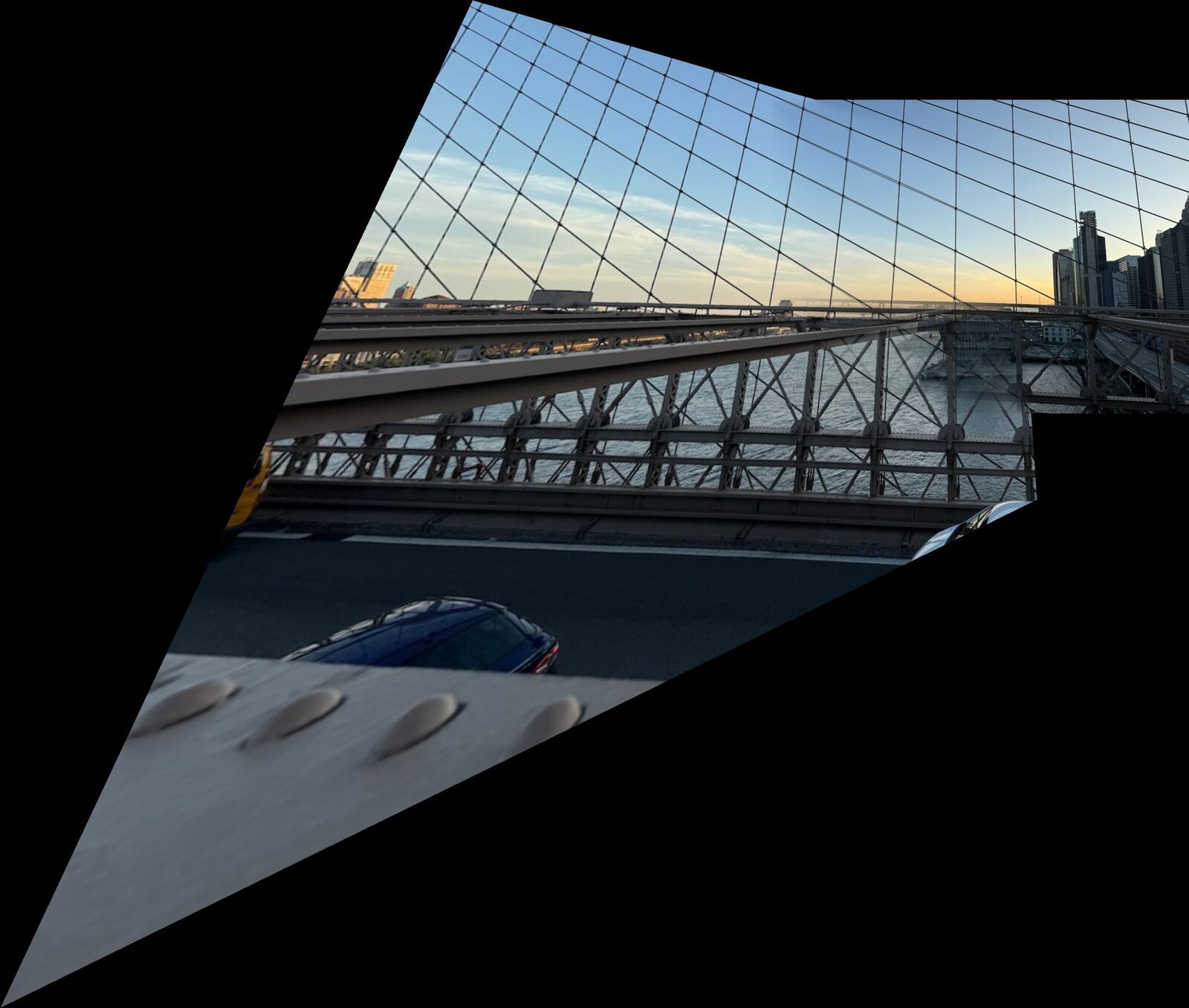
Dbridge=[1.9856953e+00−2.64638978e−01−7.3019474e+025.3917450e−011.75160307e+00−2.43720728e+021.16605560e−03−6.5845505e−041.00000000e+00] \begin{align*} D_{\text{bridge}} &= \begin{bmatrix} 1.9856953e+00 & -2.64638978e-01 & -7.3019474e+02 \\ 5.3917450e-01 & 1.75160307e+00 & -2.43720728e+02 \\ 1.16605560e-03 & -6.5845505e-04 & 1.00000000e+00 \end{bmatrix} \end{align*}

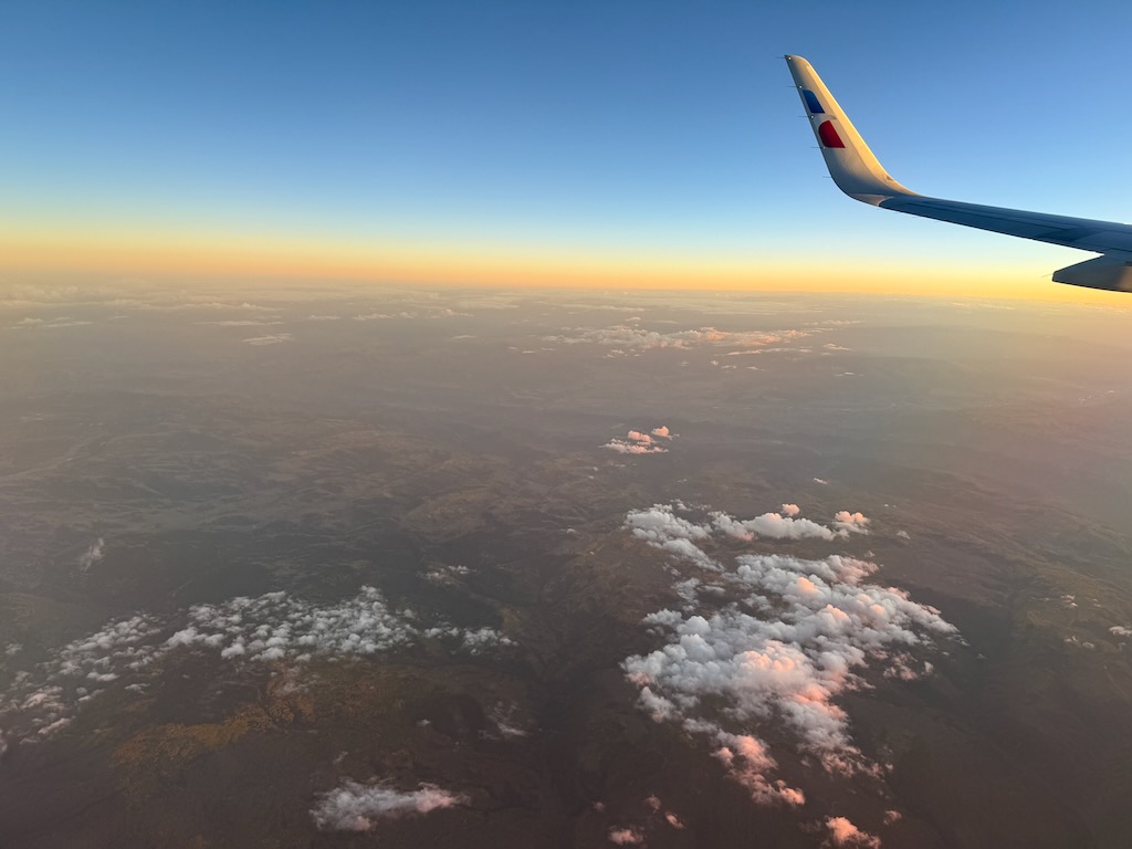
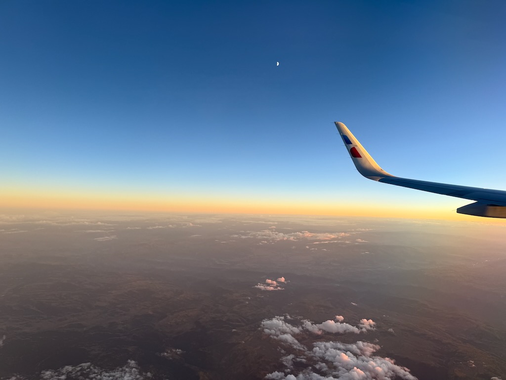
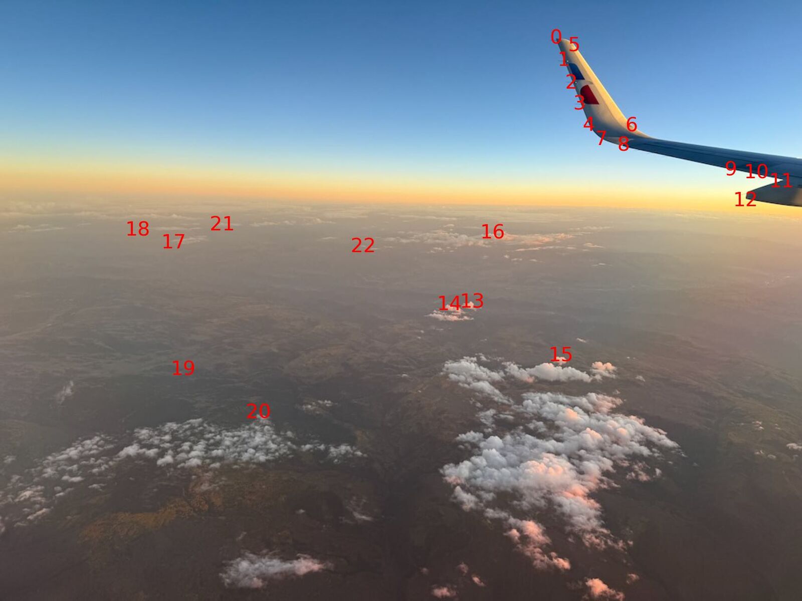
Window Seat View from NYC → SFO...

Window Seat View from NYC → SFO...

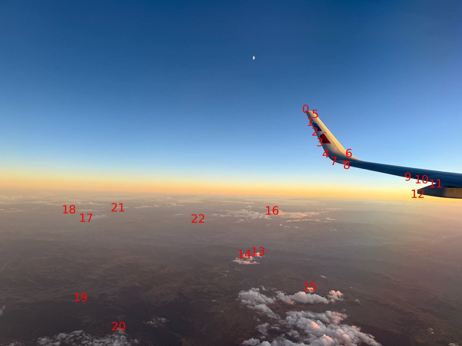
with a slightly different angle

with a slightly different angle

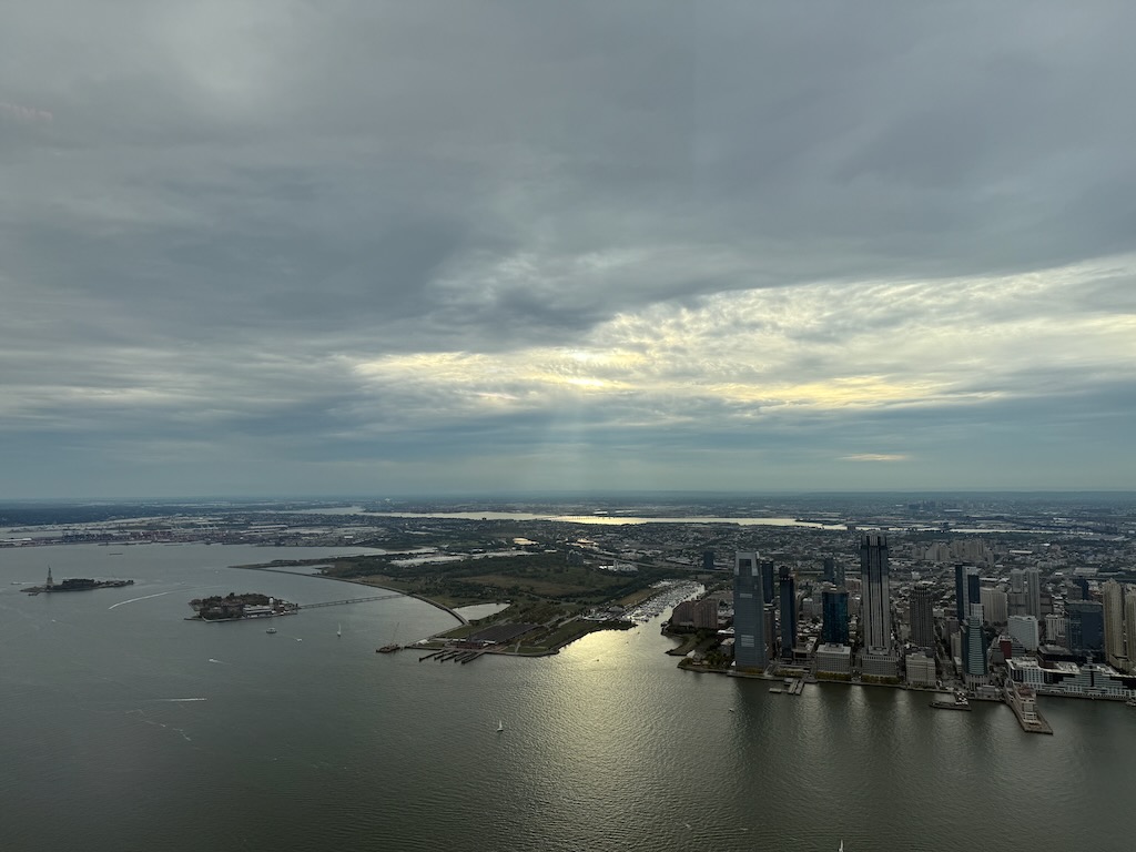
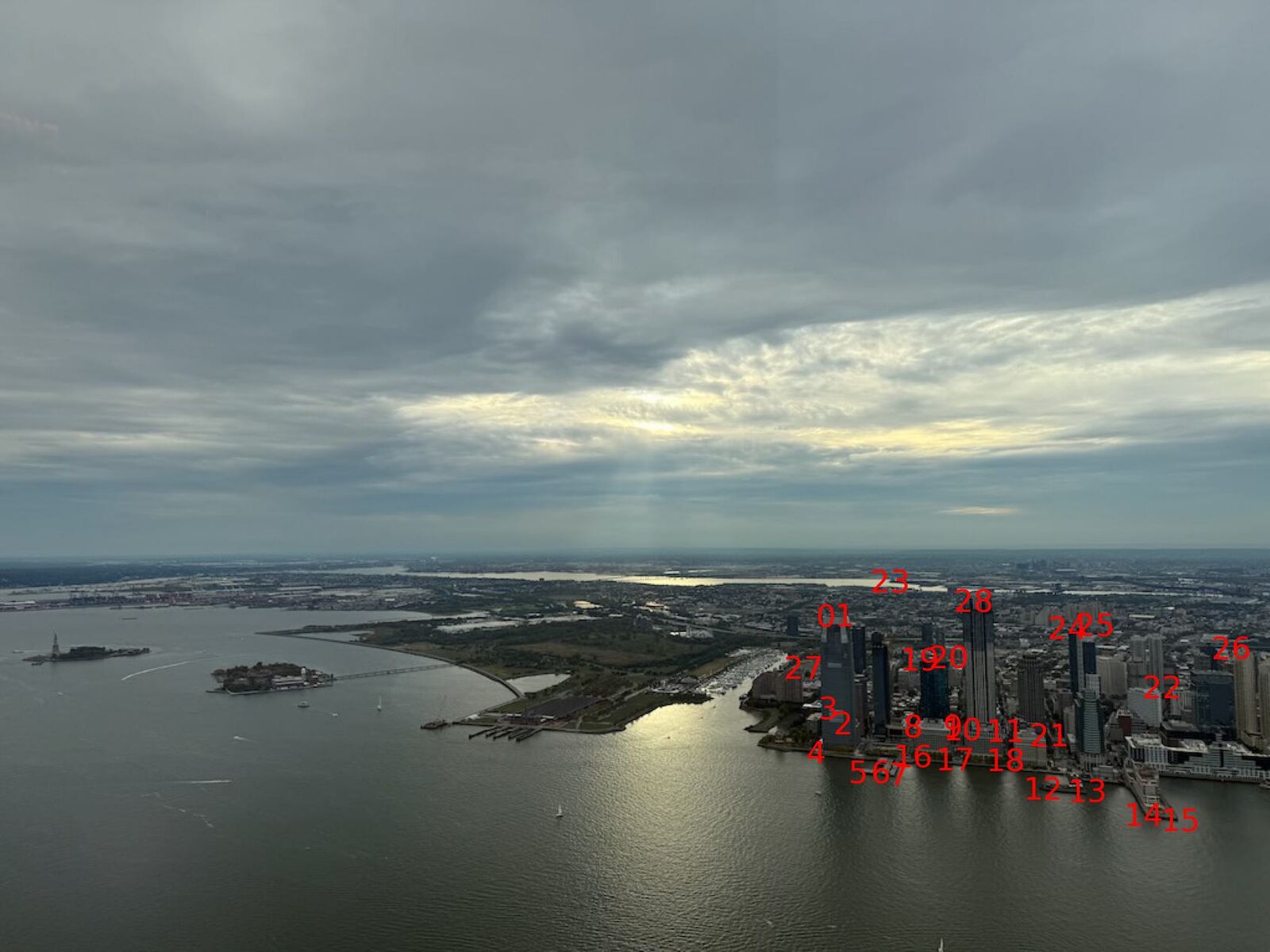
NYC from World Trade Center...

NYC from World Trade Center...

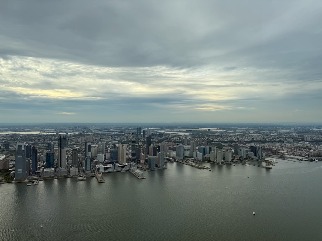
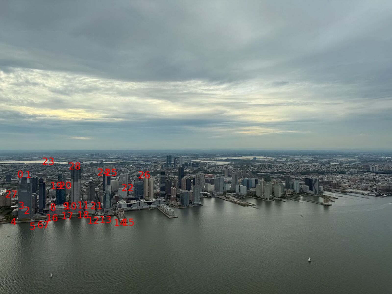
with a slightly different angle

with a slightly different angle

Point...

Point...

Correspondence

Correspondences

Point Correspondences

Point...

Correspondences

Correspondences

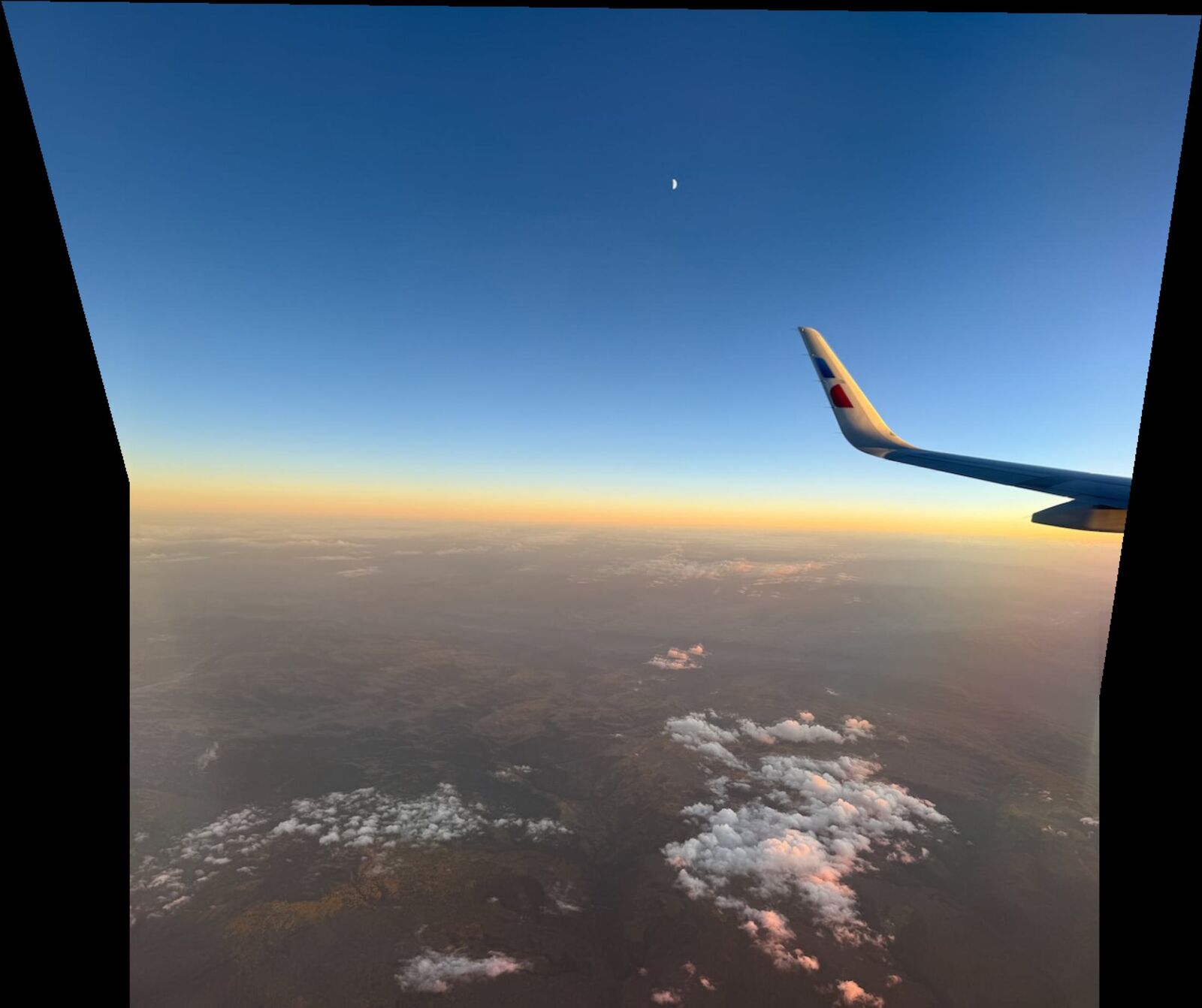
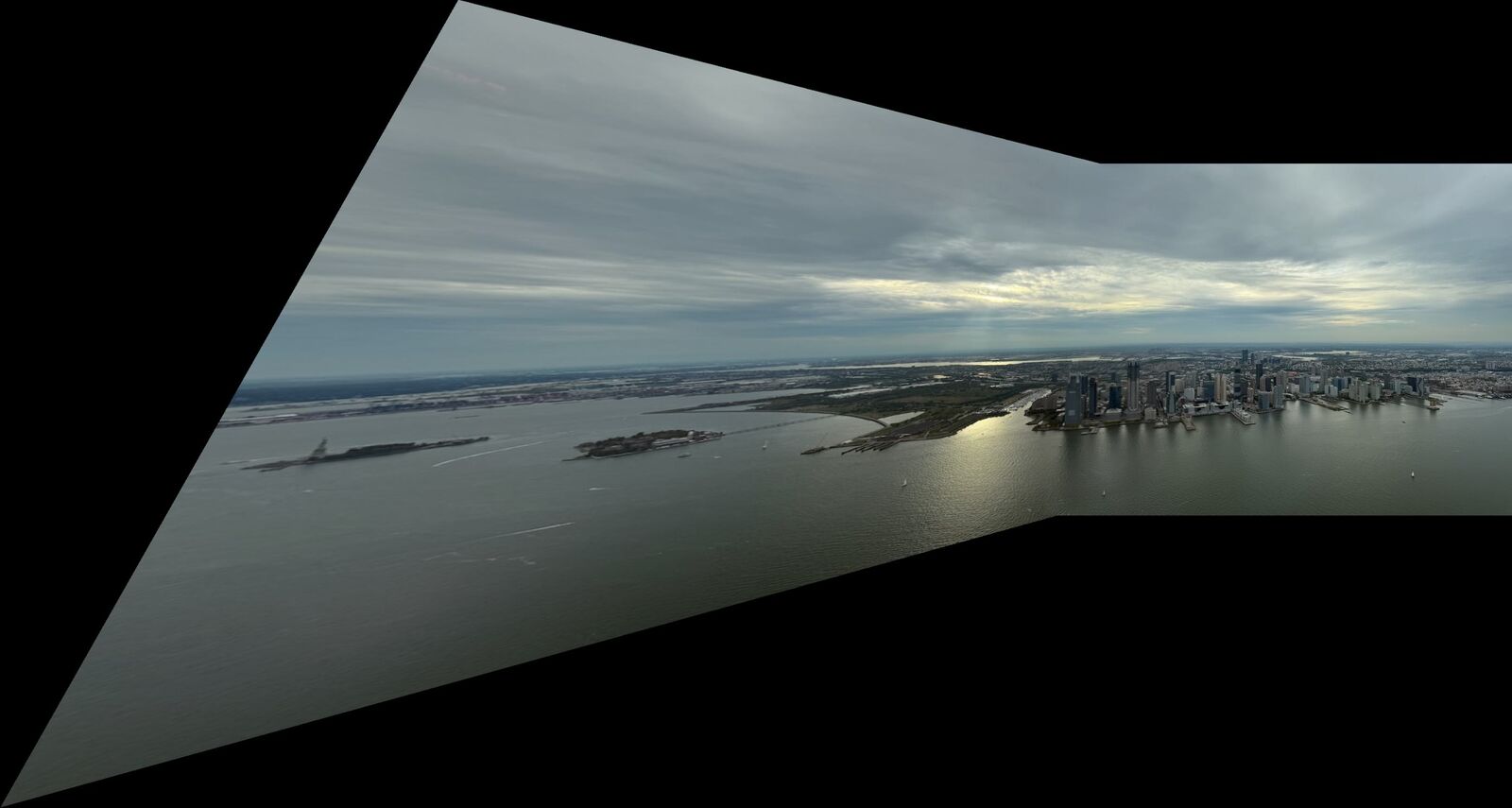
Dplane=[8.63027302e−01−2.41041893e−015.463666e+01−1.07625048e−026.9620174e−012.1719200e+02−2.462483e−05−3.74452092e−041.00000000e+00]DWTC=[2.526481e+00−1.97368342e−01−1.27606161e+035.19956729e−011.61518991e+00−3.57938253e+021.4607695e−03−4.86005876e−041.00000000e+00] \begin{align*} D_{\text{plane}} &= \begin{bmatrix} 8.63027302e-01 & -2.41041893e-01 & 5.463666e+01 \\ -1.07625048e-02 & 6.9620174e-01 & 2.1719200e+02 \\ -2.462483e-05 & -3.74452092e-04 & 1.00000000e+00 \end{bmatrix} \\ \\ D_{\text{WTC}} &= \begin{bmatrix} 2.526481e+00 & -1.97368342e-01 & -1.27606161e+03 \\ 5.19956729e-01 & 1.61518991e+00 & -3.57938253e+02 \\ 1.4607695e-03 & -4.86005876e-04 & 1.00000000e+00 \end{bmatrix} \end{align*}

A.3: Warp the Images

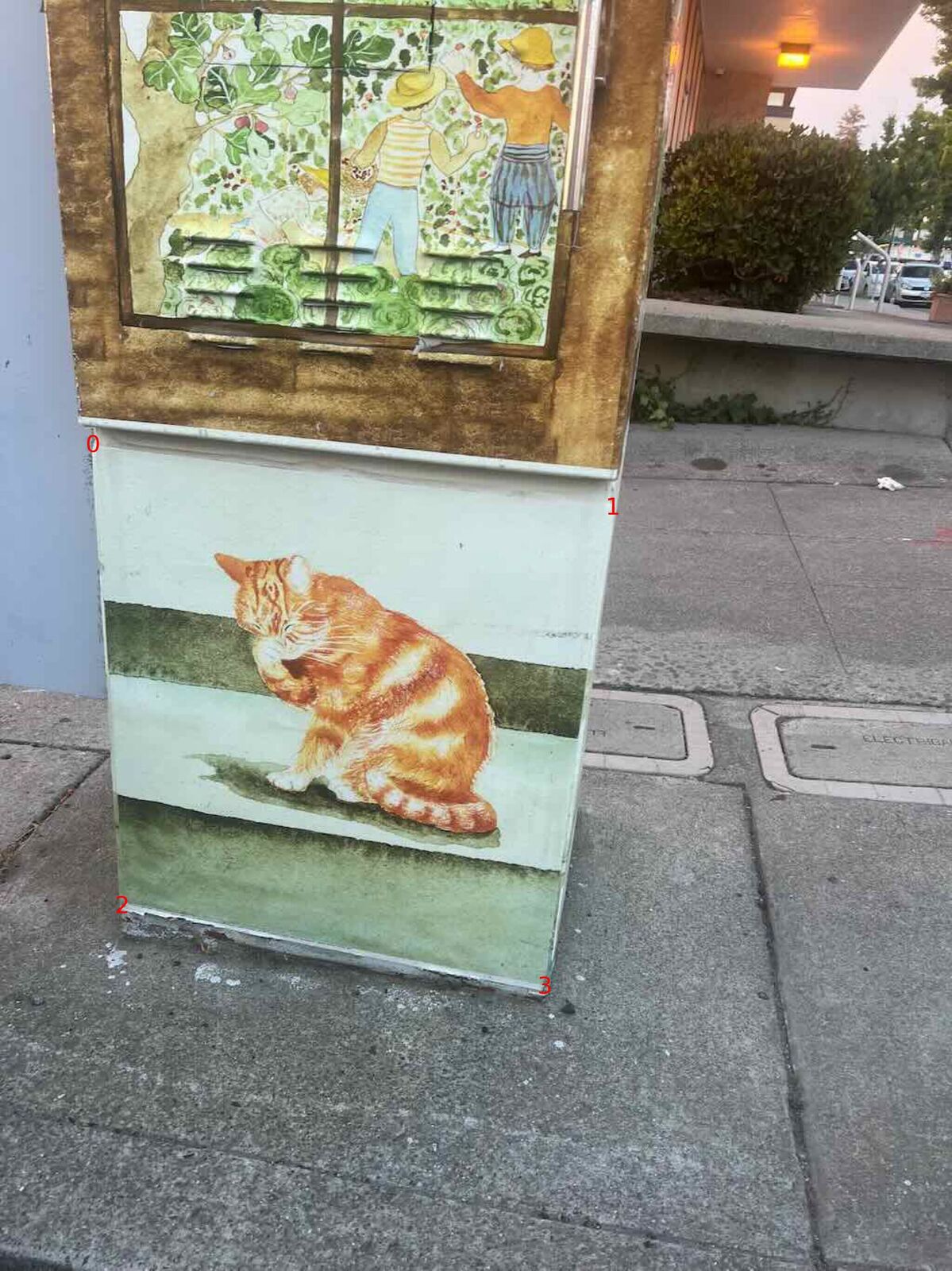
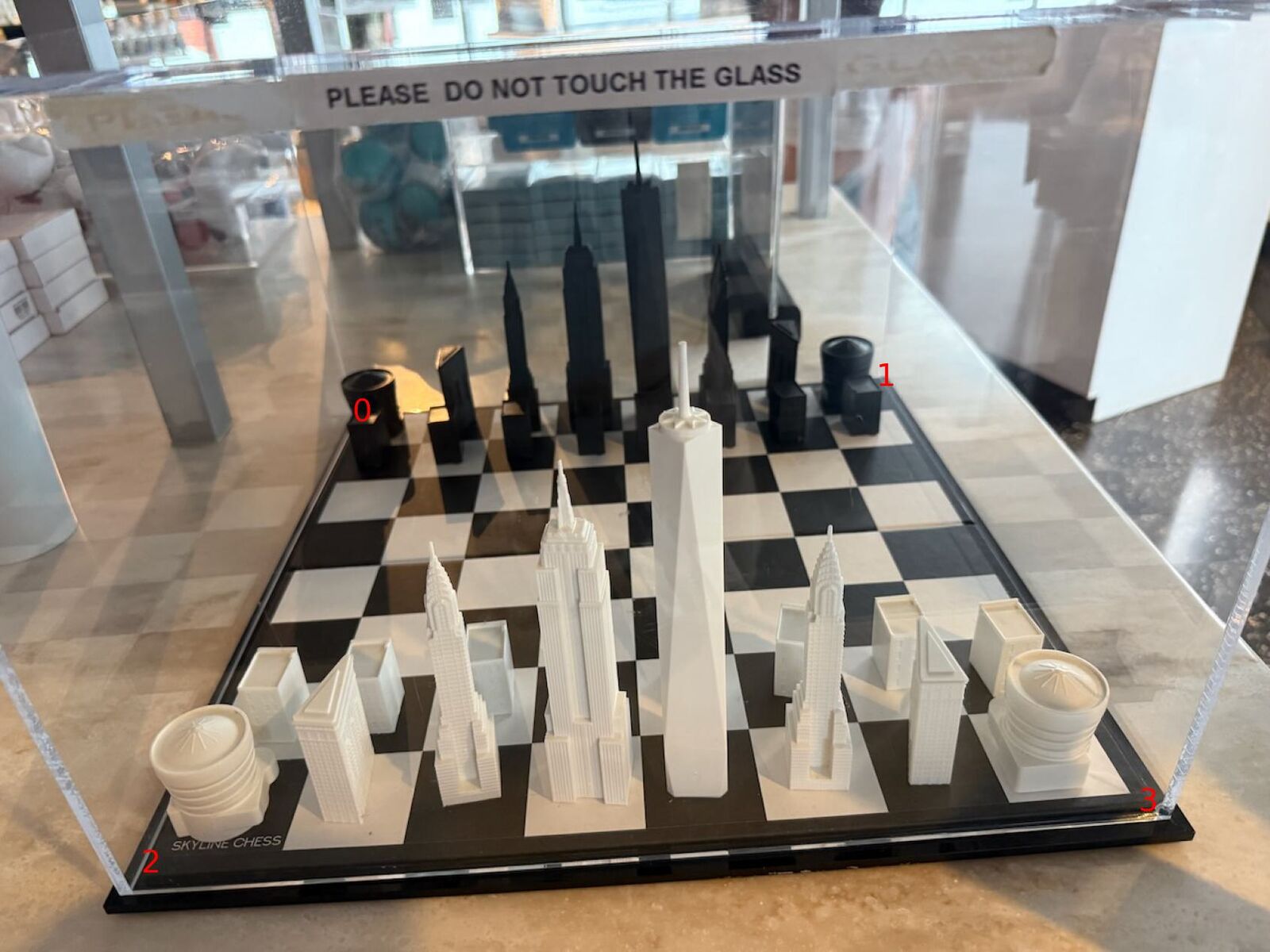
Rectification:
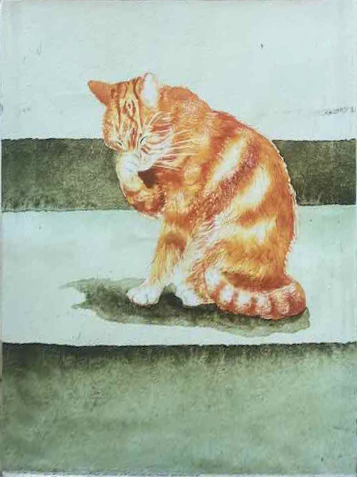
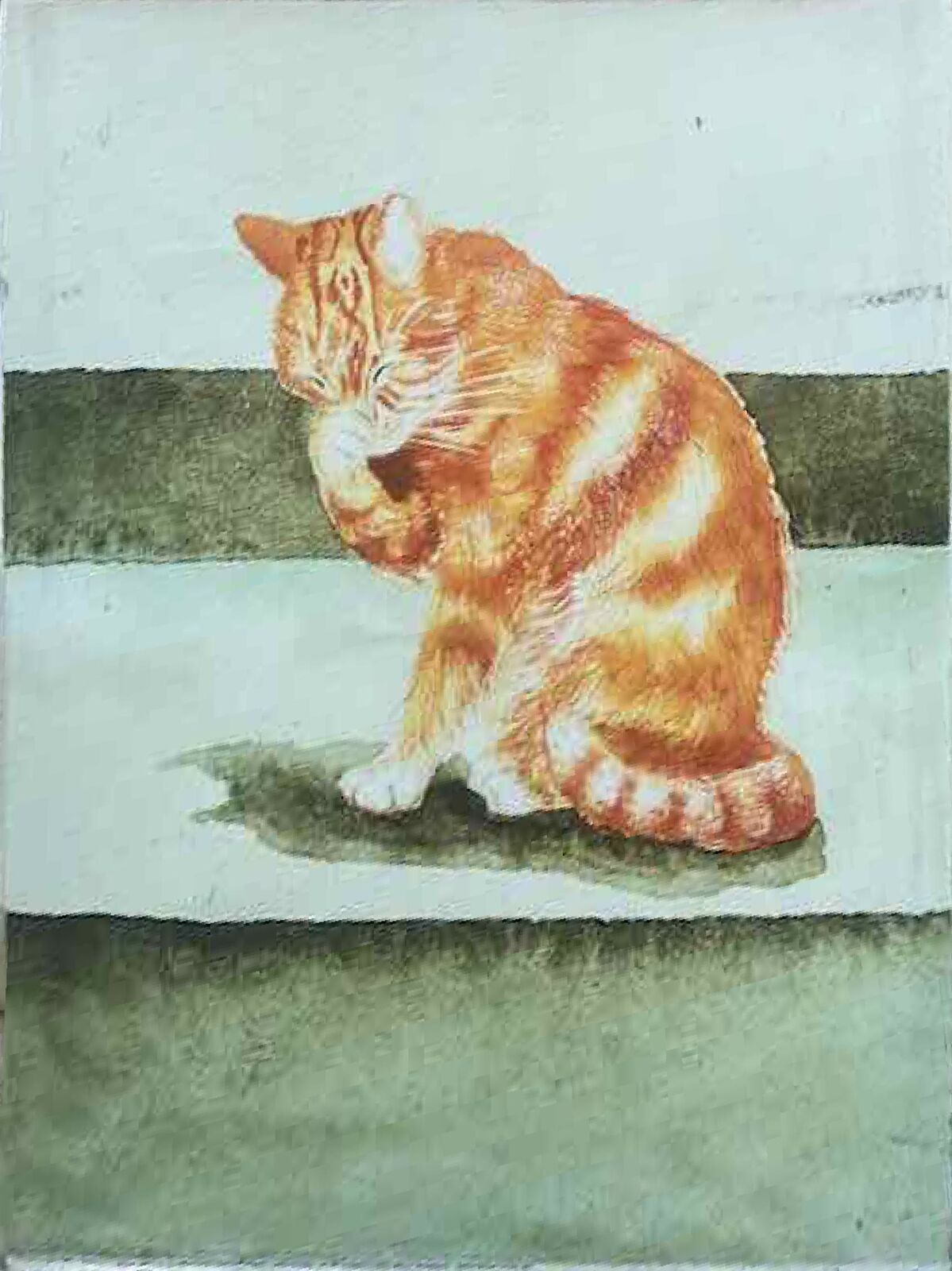
Cat Mural (Berkeley, CA)

Cat Mural (Berkeley, CA)

Bilinear
Nearest Neighbors
↔

Nearest Neighbor vs Bilinear Interpolation

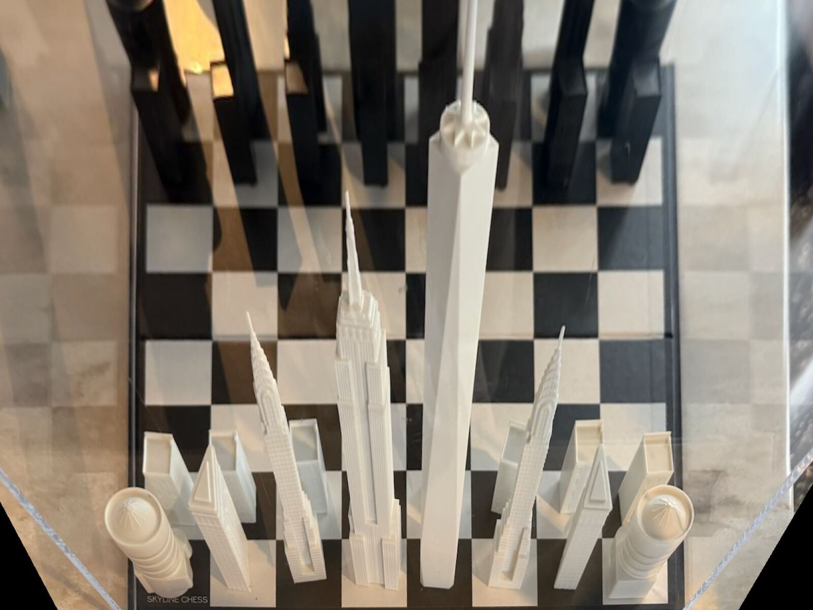
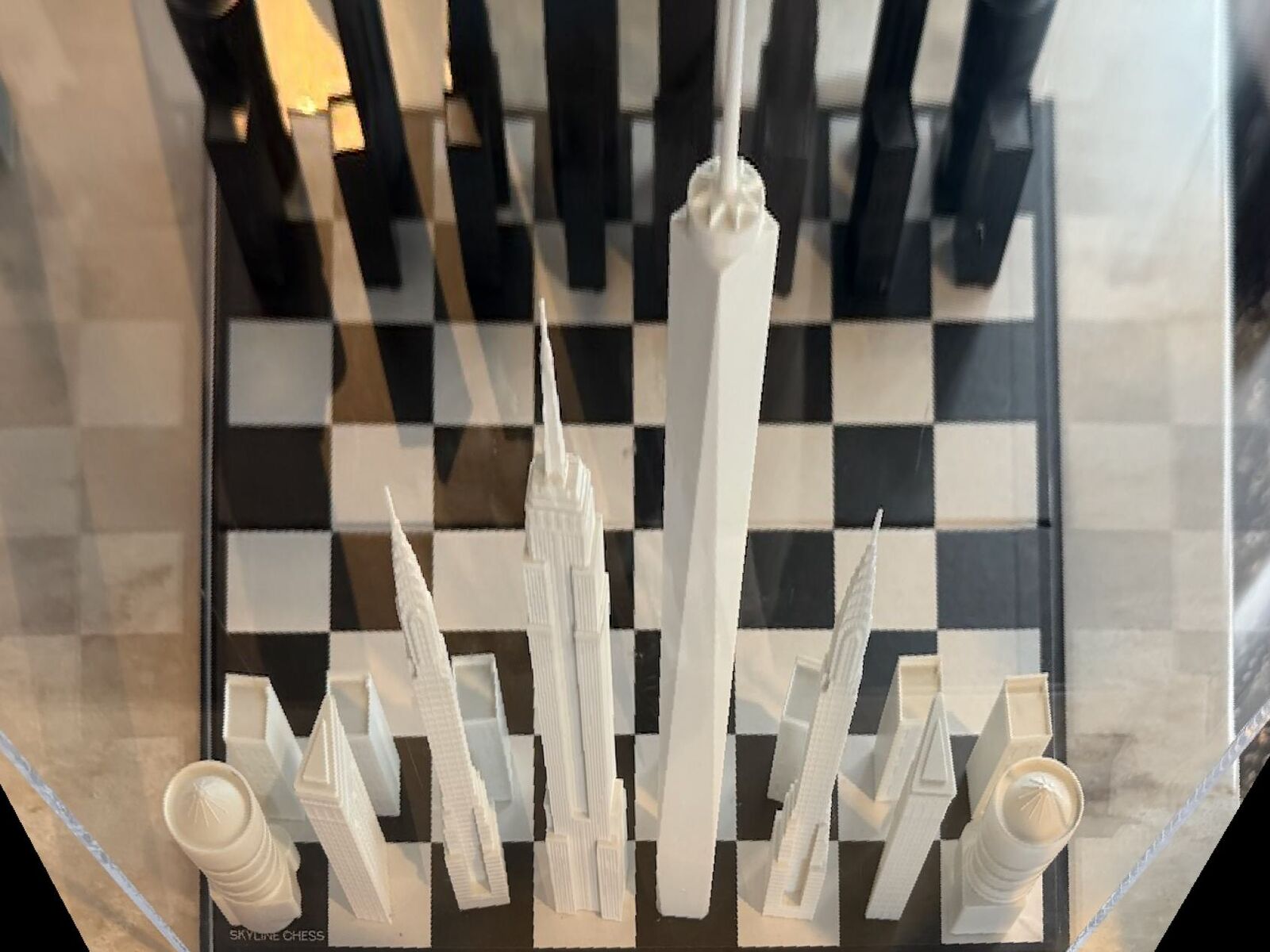
3D-Printed Chess Board (World Trade Center, NY)

3D-Printed Chess Board (World Trade Center, NY)

Bilinear
Nearest Neighbors
↔

Nearest Neighbor vs Bilinear Interpolation

A.4: Blend the Images into a Mosaic

Process:

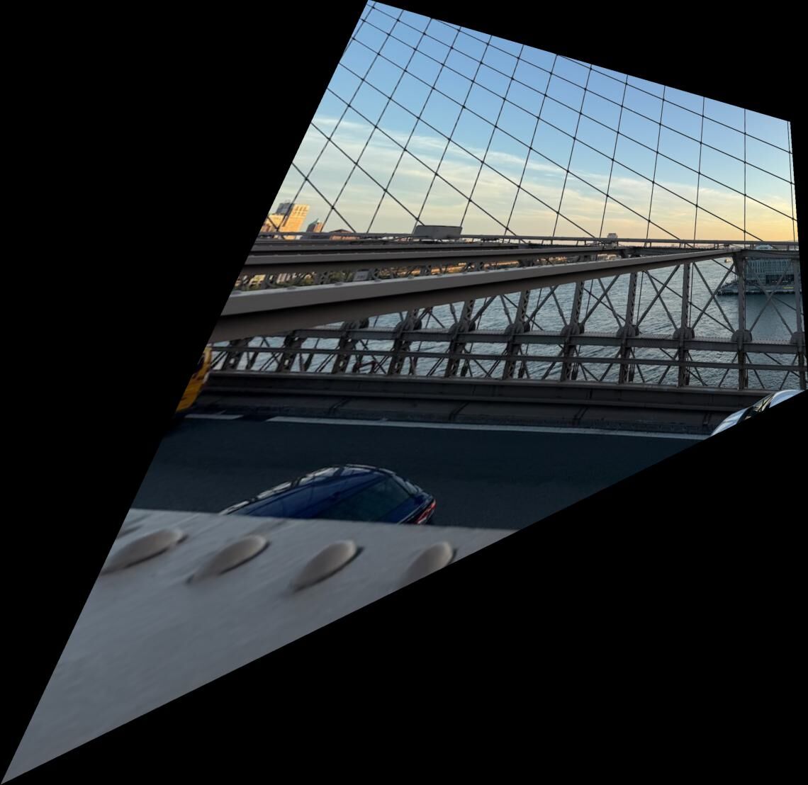
  1. Warp Image 1
    Warped Image 1
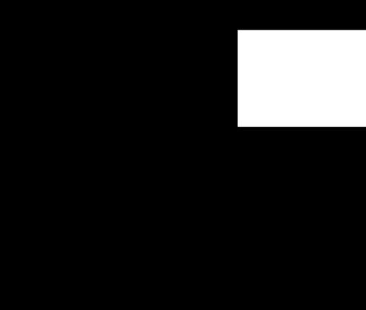
  2. Initialize mask to 1 where image has nonzero pixels and 0 elsewhere

    mask1

    mask2

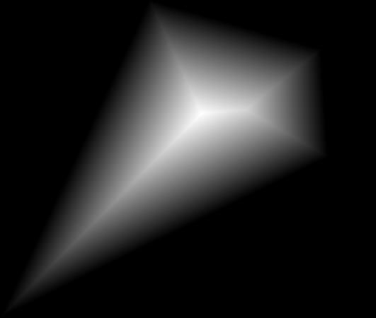
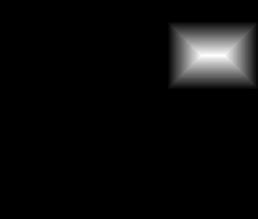
  3. Use scipy's ndimage.distance_transform_edt to create blurring mask

    (maps each nonzero pixel value to the distance between it and the nearest zero value)

    dist_transform1

    dist_transform2

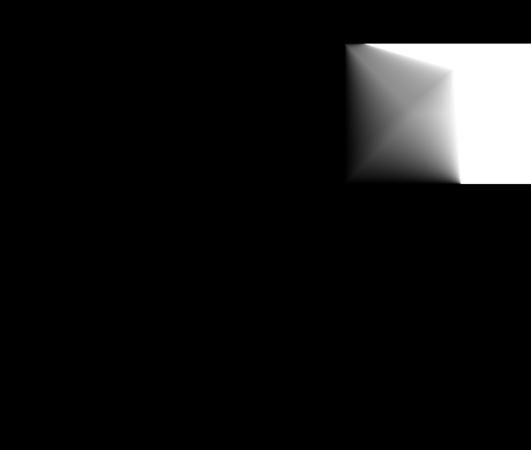
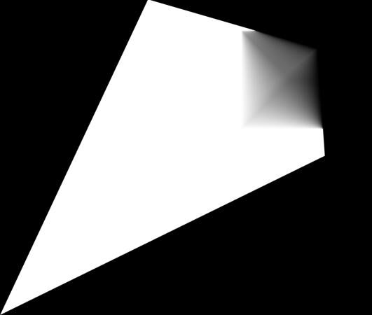
  4. Manually set blurring masks to original mask values (1 and 0) where the masks do not overlap
    weight2
    weight1
    ↔
  5. output = weight1 * warped1 + weight2 * image2
    Brooklyn Bridge Mosaic

    Brooklyn Bridge Mosaic

Other examples:

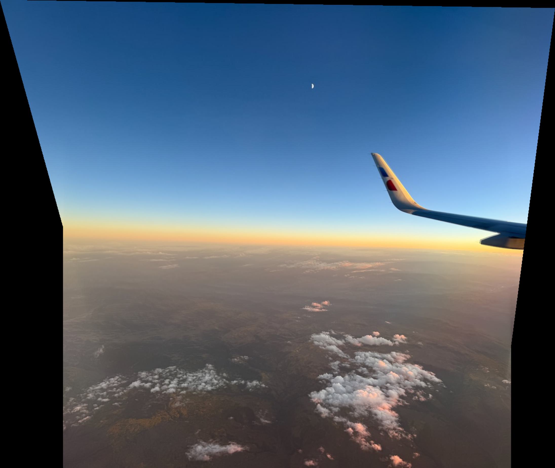
Plane View Mosaic

Plane View Mosaic

World Trade Center Mosaic

World Trade Center Mosaic

Feature Matching for Autostitching

B.1: Harris Corner Detection

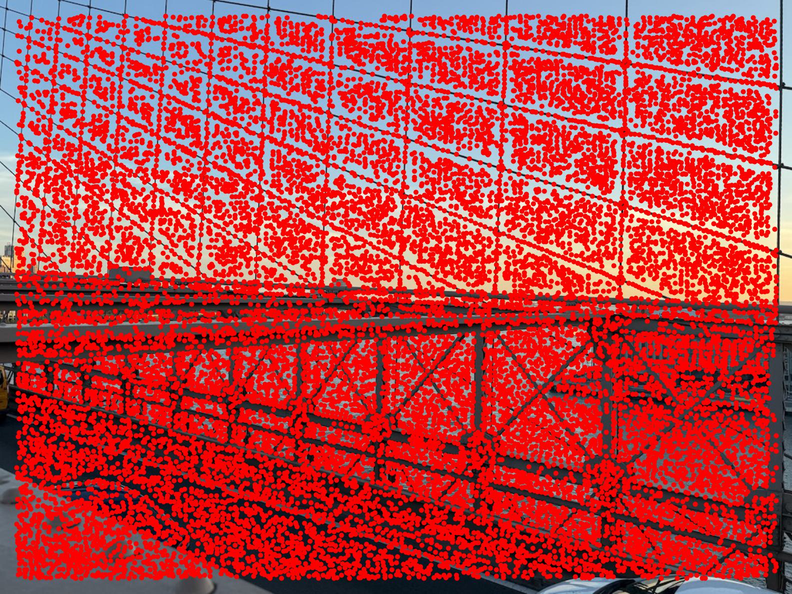
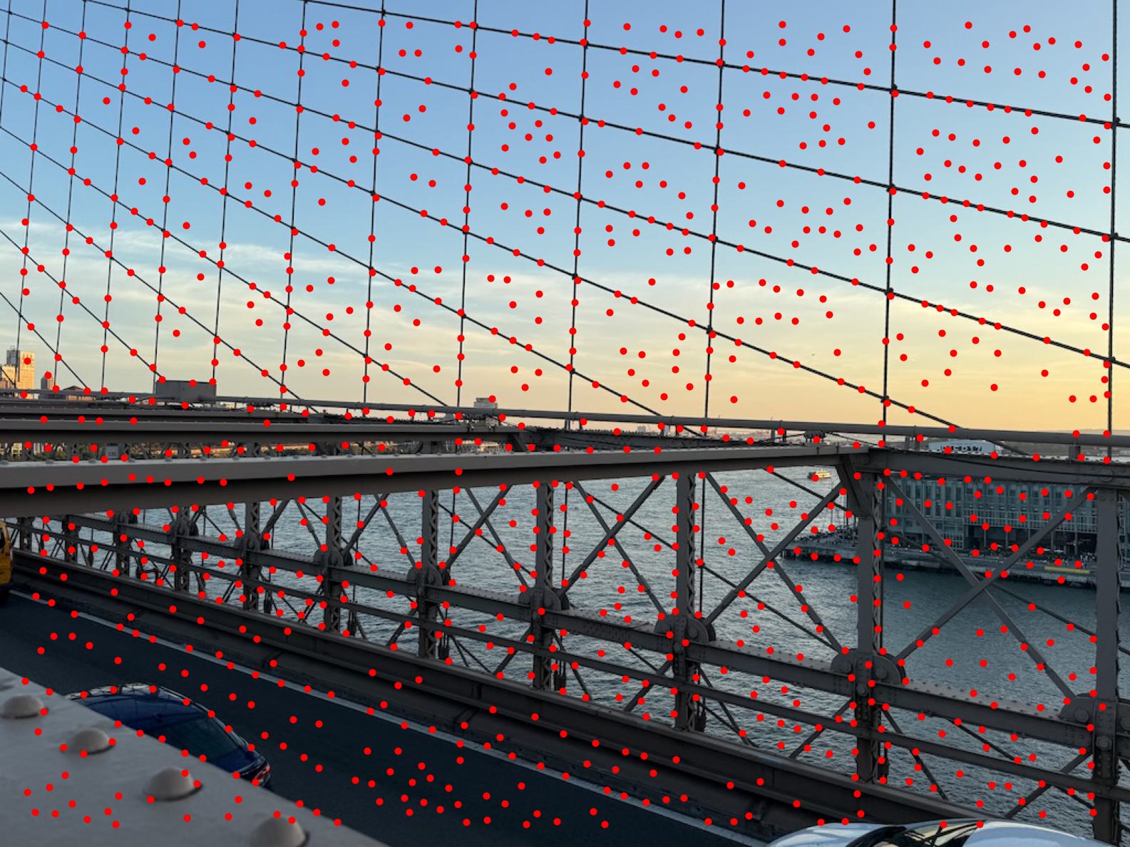
Detected Harris corners without ANMS

Detected Harris corners without ANMS

Detected Harris corners without ANMS

Detected Harris corners without ANMS

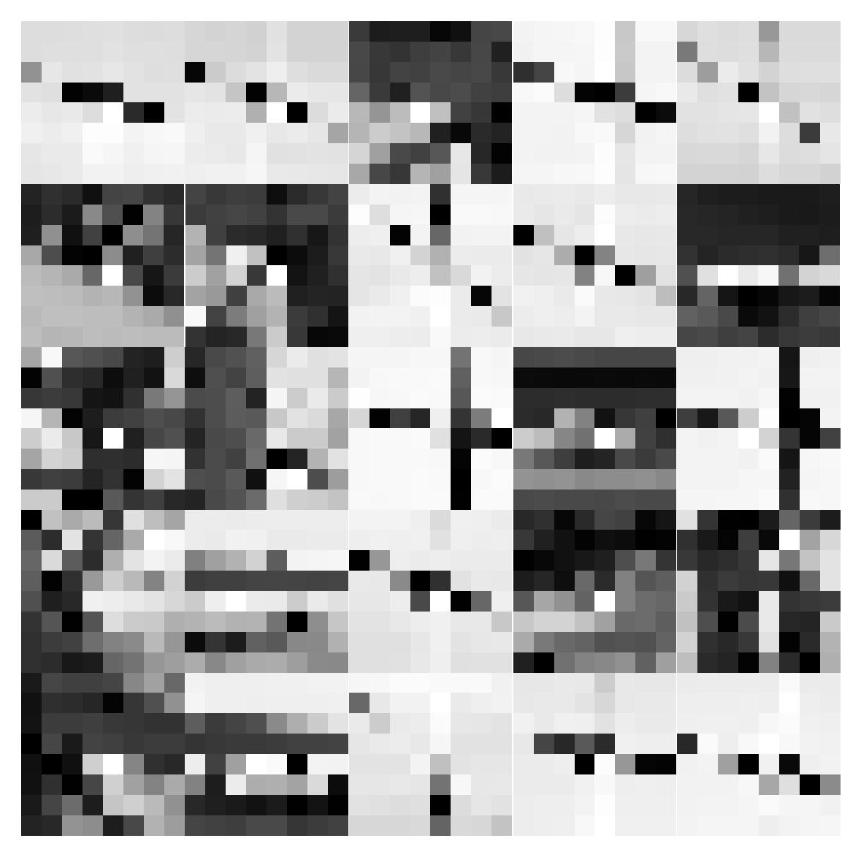
B.2: Feature Descriptor Extraction

Normalized Extracted Features with ANMS

Normalized Extracted Features (after ANMS)

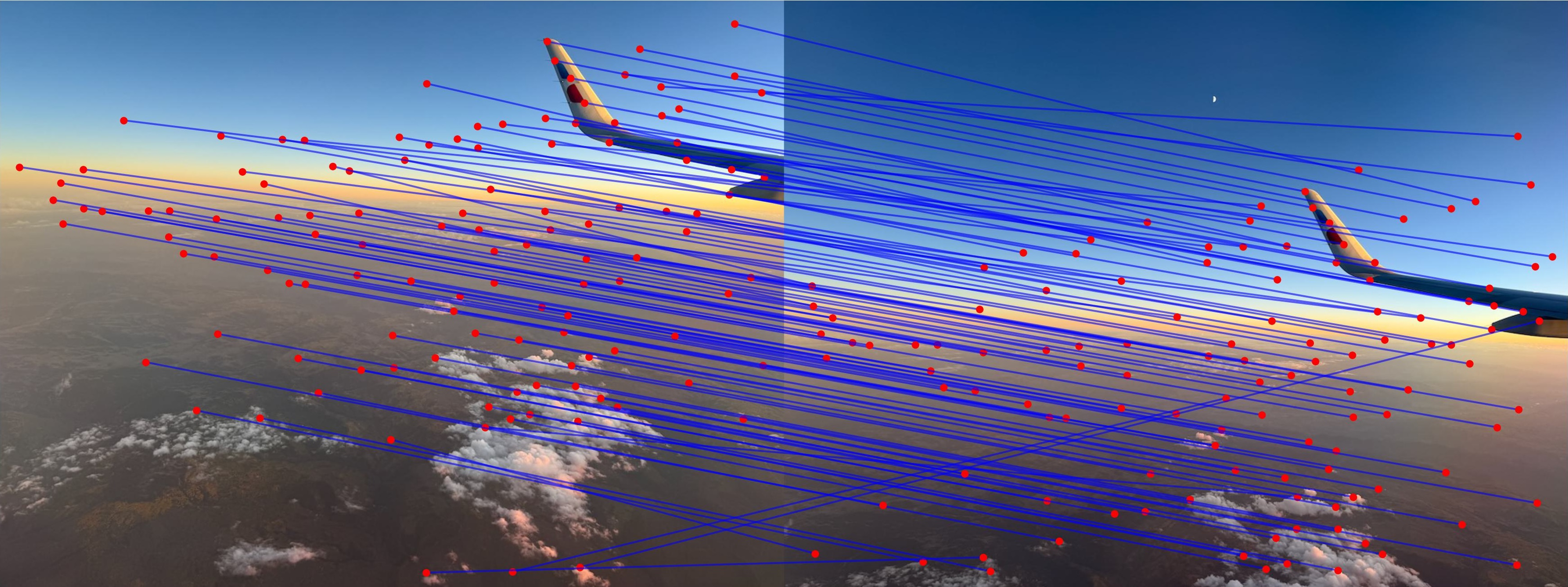
B.3: Feature Matching

Matched Features

Matched Features

B.4: RANSAC for Robust Homography

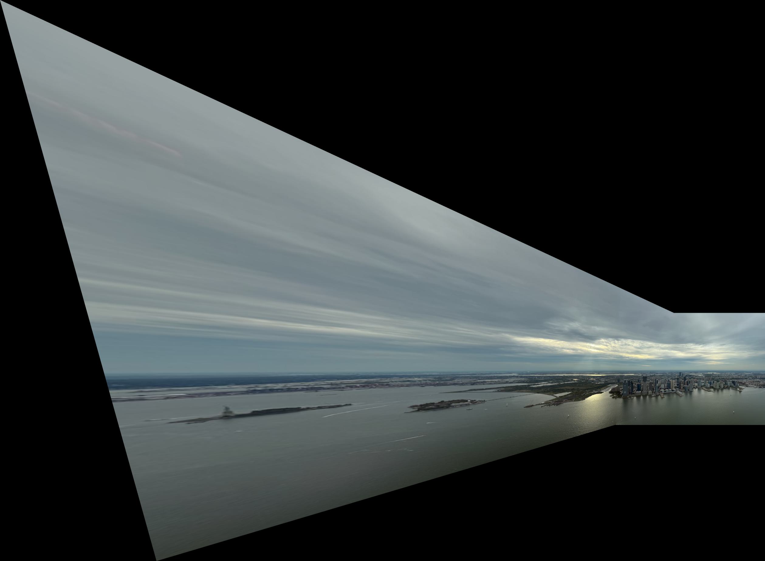
World Trade Center Mosaic from Manually-selected Features

World Trade Center Mosaic from Manually-selected Features

World Trade Center Mosaic from Auto-detected Features

World Trade Center Mosaic from Auto-detected Features:
Even though the final mosaics were different, they both seemed to capture the overall scene.

Plane View Mosaic from Manually-selected Features

Plane View Mosaic from Manually-selected Features

Plane View Mosaic from Auto-detected Features

Plane View Mosaic from Auto-detected Features

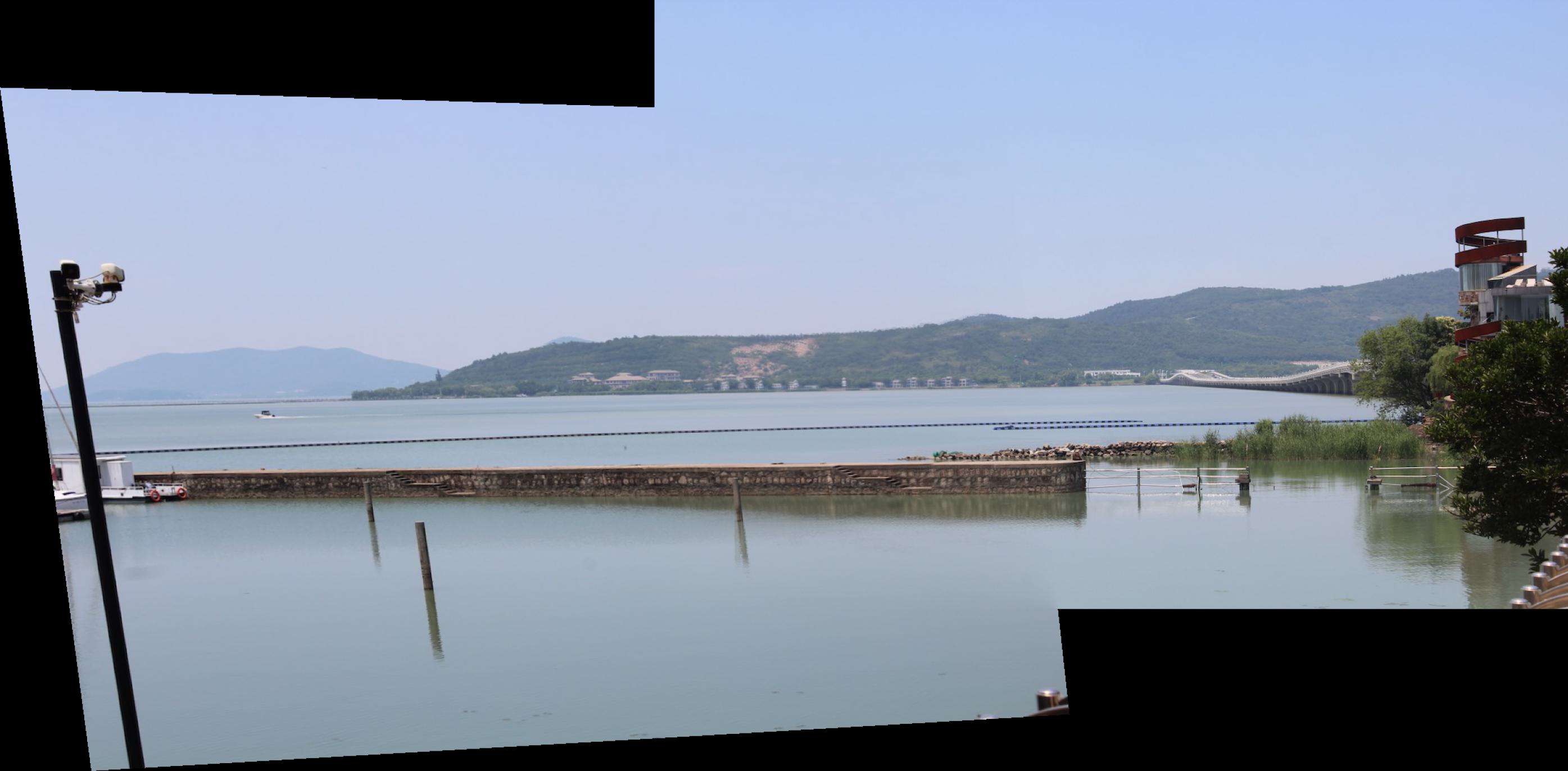
TaiEr, China Mosaic from Manually-selected Features

TaiEr, China Mosaic from Manually-selected Features

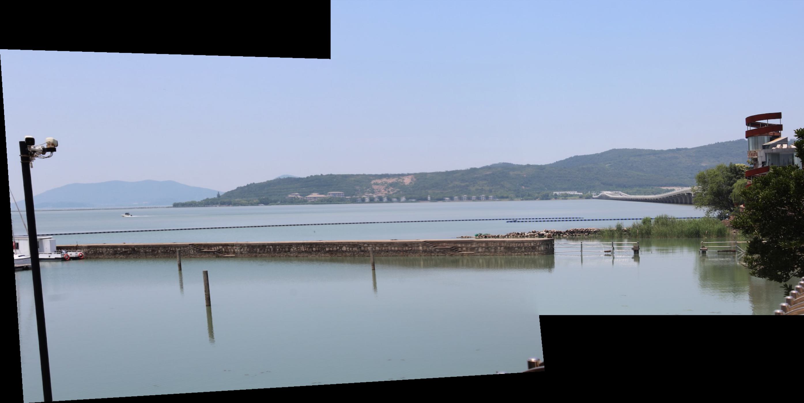
TaiEr, China Mosaic from Auto-detected Features

TaiEr, China Mosaic from Auto-detected Features

Failed Examples

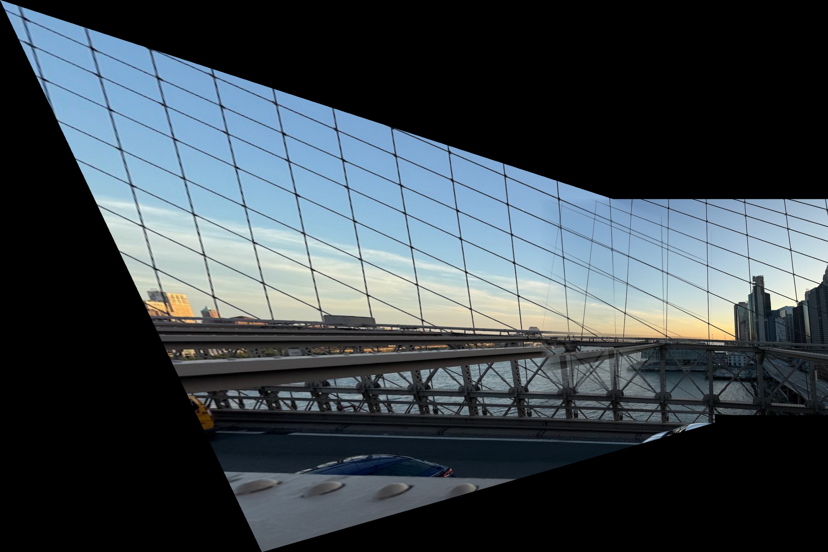
Brooklyn Bridge Mosaic from Auto-detected Features

Brooklyn Bridge Mosaic from Auto-detected FeaturesIt was difficult for the RANSAC Algorithm to find the correct homography because Brooklyn Bridge image has a largely repeating pattern of wires. While it is easy for humans to identify the corresponding features, the algorithm struggles to find them due to the similarity of the features our algorithm can extract.