Project 2: Fun with Filters and Frequencies
September 26, 2025
Overview
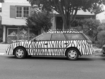
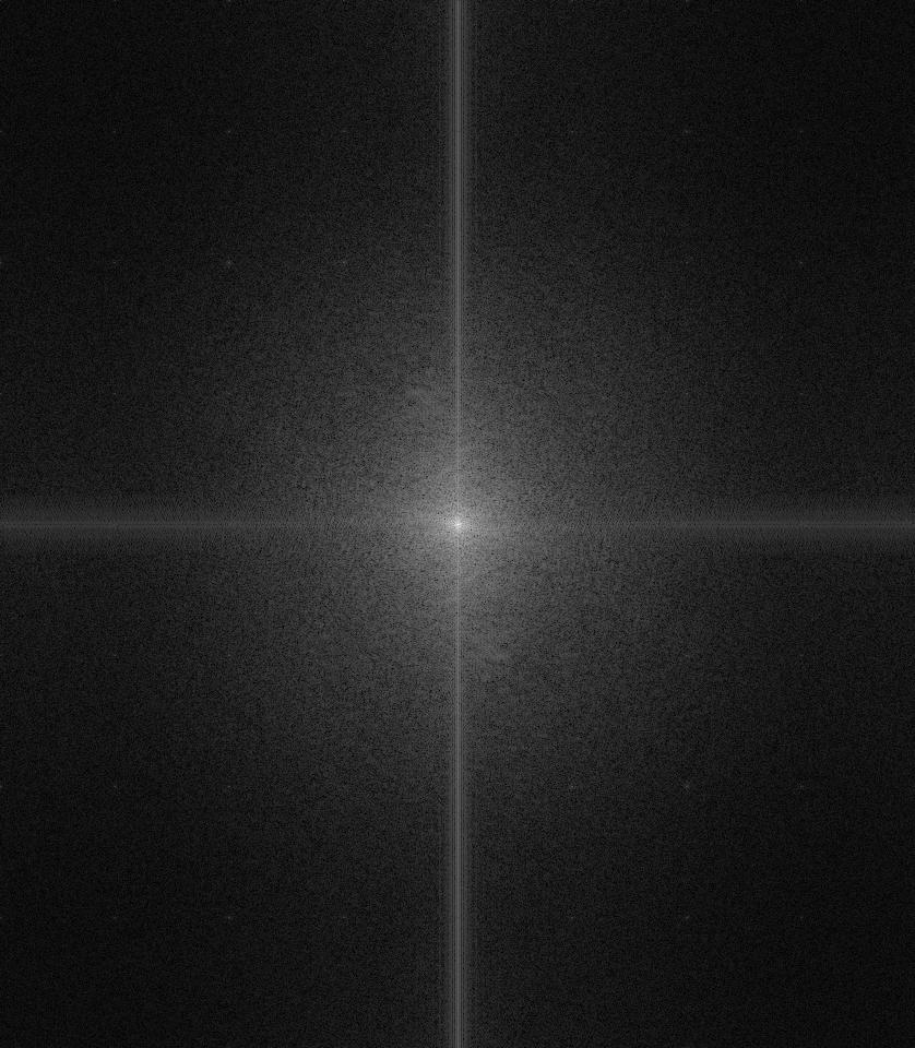
A zebra car I saw on my run in spatial domain
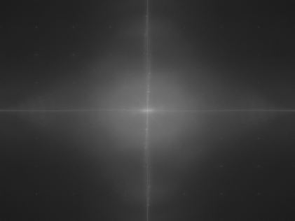
...vs frequency domain
Understanding images from a frequency perspective rather than spatial perspective is crucial in digital image processing. Images are made up of different frequency components, with low frequencies capturing the general structure of an image and high frequencies capturing small/fine details. By manipulating the constituent frequencies of images, we can blur, sharpen, and blend images seamlessly.
The goal of this assignment is to demonstrate how image processing in the frequency domain can be used to achieve interesting visual effects.
Convolutions
1.1 From Scratch!
Mathematically, convolution is defined as:
Convolution is an associative and communative operation, i.e.
Let's take a look at what convolution does!
The following are a couple of filters/kernels:
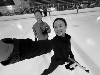
Original Image (): my sister and I skating together again!
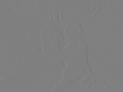
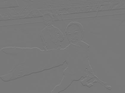
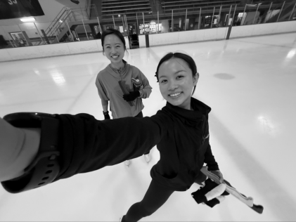
* Should look blurry, but here, it is still relatively clear since the kernel (3x3) is small compared to my image
Code Implementation
In practice, convolution is a very commonly used operation, leading to many performance optimizations (through formulation of convolution as matrix-multiplication followed by parallelization) Let's compare the runtime it takes to convolve an image and filter using SciPy's convolve2d, a function from a prebuild library, with two naive implementations.
Scipy convolution time: 0.1677 seconds
VERSUS
def convolve_four_loops(image, kernel):

  ... (handling of padding) ...
  # In my implementation, I used zero-padding, i.e. just add zeros to the edge of the original image
  # But I found that when using Sci-py's convolve2d, 'symm' padding, i.e. mirror the edge pixels,
  # was the best for the processing I was doing

  for i in range(ih):
      for j in range(iw):
          sum = 0
          for m in range(kh):
              for n in range(kw):
                  sum += kernel[m, n] * padded_image[i + m, j + n] # this is scalar multiplication
          output[i, j] = sum

return outputdef convolve_two_loops(image, kernel):
... (handling of padding) ...
for i in range(ih):
for j in range(iw):
region = padded_image[i:i+kh, j:j+kw]
output[i, j] = np.sum(region * kernel) # this is element-wise multiplication followed by sum of all elements
return outputFilters!
1.2 Finite Difference Operator
The finite difference operator is a simple filter that approximates the derivative of an image in a specific direction. i.e.
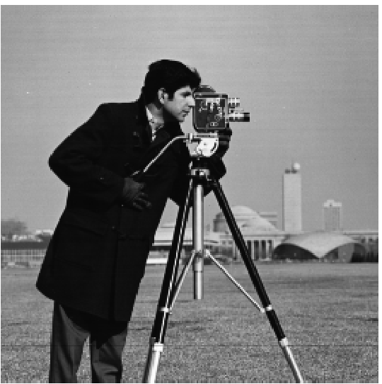
Original Image (): "camera_man.png"
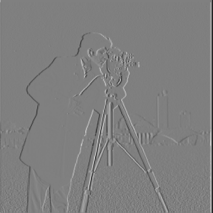
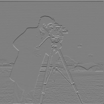
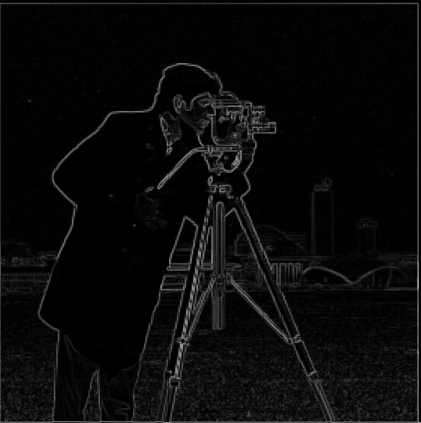
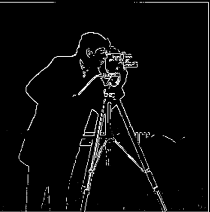
(thresholded gradient magnitude)
* Note how the thresholded gradient magnitude image clearly highlights the strong edges in the image.
1.3 Derivative of Gaussian (DoG) Filters
In real-world images, noise can create false edges and make it difficult to accurately detect true edges. To mitigate this, we can smooth the image using a Gaussian filter before applying the derivative operator. This combination (of Gaussian smoothing and finite difference operator) is known as the Derivative of Gaussian (DoG) filter.
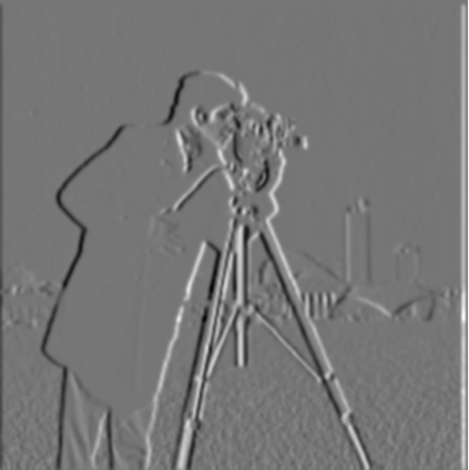
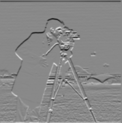
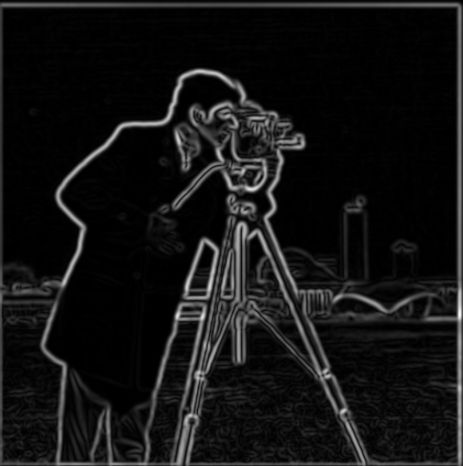
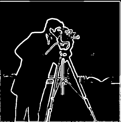
(thresholded gradient magnitude)
Comparing these derivatives and magnitudes with those from a plain Finite Difference Operator convolution, we can see how DoG creates a more robust edge detection filter.
To understand why the Derivative of Gaussian (DoG) filter reduces high-frequency noise while preserving important low-frequency structures in the image (thus making edges more distinct), let's break down the process into two steps:
- smoothing the image to reduce noise that obscures or distracts from edges (remove high-frequencies)
- applying a derivative operation on the smoothed image to detect edges.
Max difference in X derivatives: 0.004088
Max difference in Y derivatives: 0.004337
* I chose and a (to capture 99% of the Gaussian distribution) for the above results because it seemed to get rid of enough noise while preserving the low-frequency edges of the camera-man.
** To choose the thresholds for the gradient magnitude, I tried a few values and chose the ones that seem to throw away all the background (e.g. grass) and keep the edges of the camera-man.
Image "Sharpening"
2.1 How it works
The Gaussian filter we used earlier acts as low pass filter that retains only the low frequencies. If we subtract the blurred version (only low frequencies) from the original image, we get the high frequencies of the image. An image often looks "sharper" if it has more high frequencies, so we can make images look "sharper" by adding these high frequencies to the original image.
Let's visualize the process of the unsharp filter (from left to right):
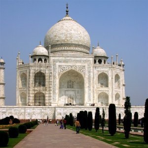
Original Image (): "taj_mahal.jpg"
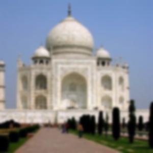
(Low Frequencies)
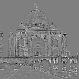
(High Frequencies)
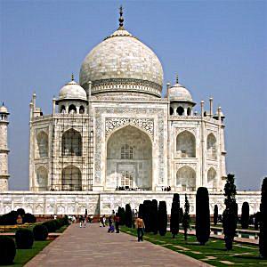
(Sharpened with )
Unsharp Mask Filter
We can also combine this process into a single convolution operation called the unsharp mask filter.
Let denote a grayscale 2D image, denote the sharpening parameter, denote a Gaussian filter, and denote a 2-D unit impulse. Starting from the definition of the unsharp procedure, we apply the properties of convolution to get a single convolution operation:
Visualizing the effects of the sharpening parameter,
denotes the sharpening parameter, i.e. the "strength" of sharpening. The larger the , the more of the high-frequency components we are adding, creating a stronger sharpening effect.
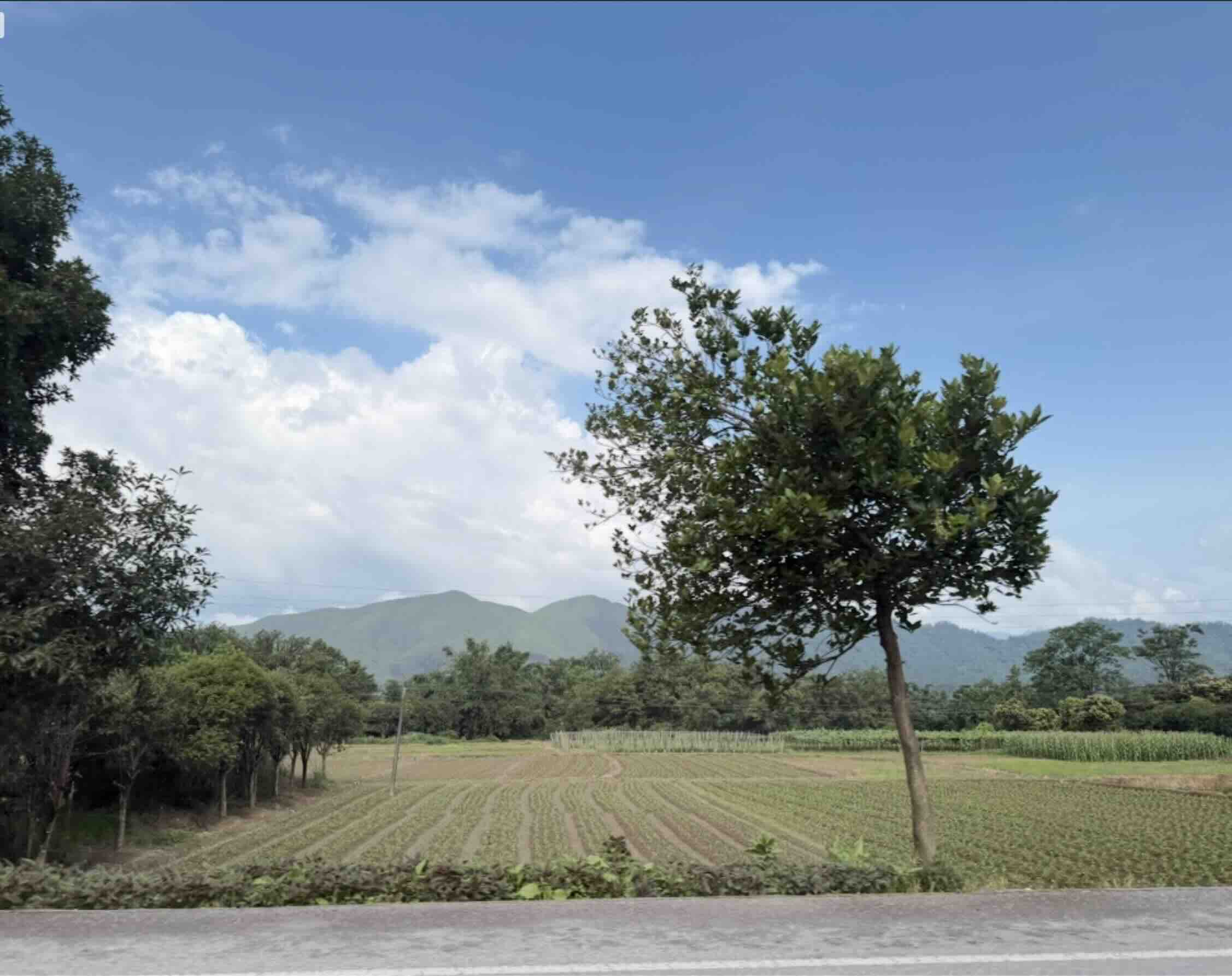
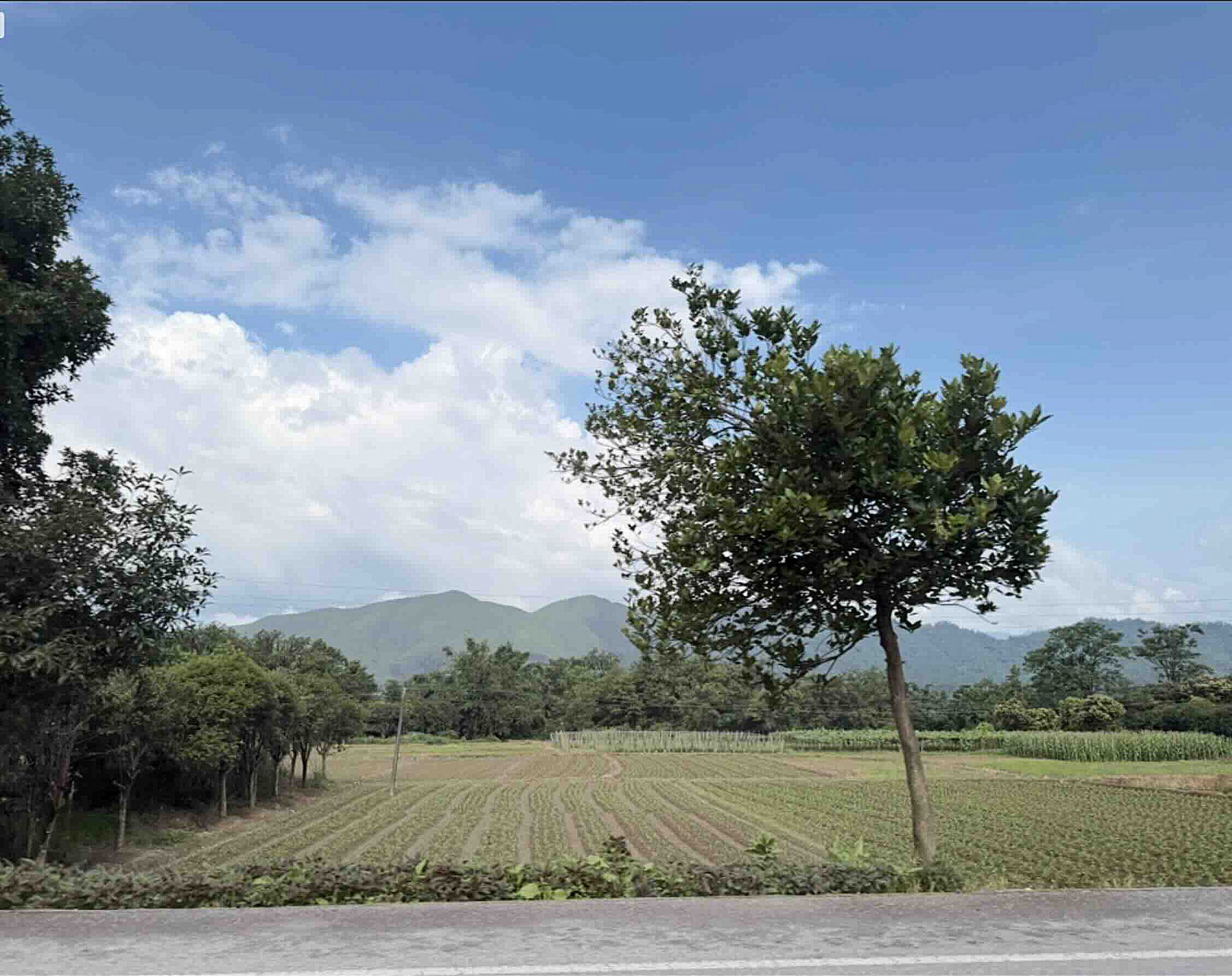
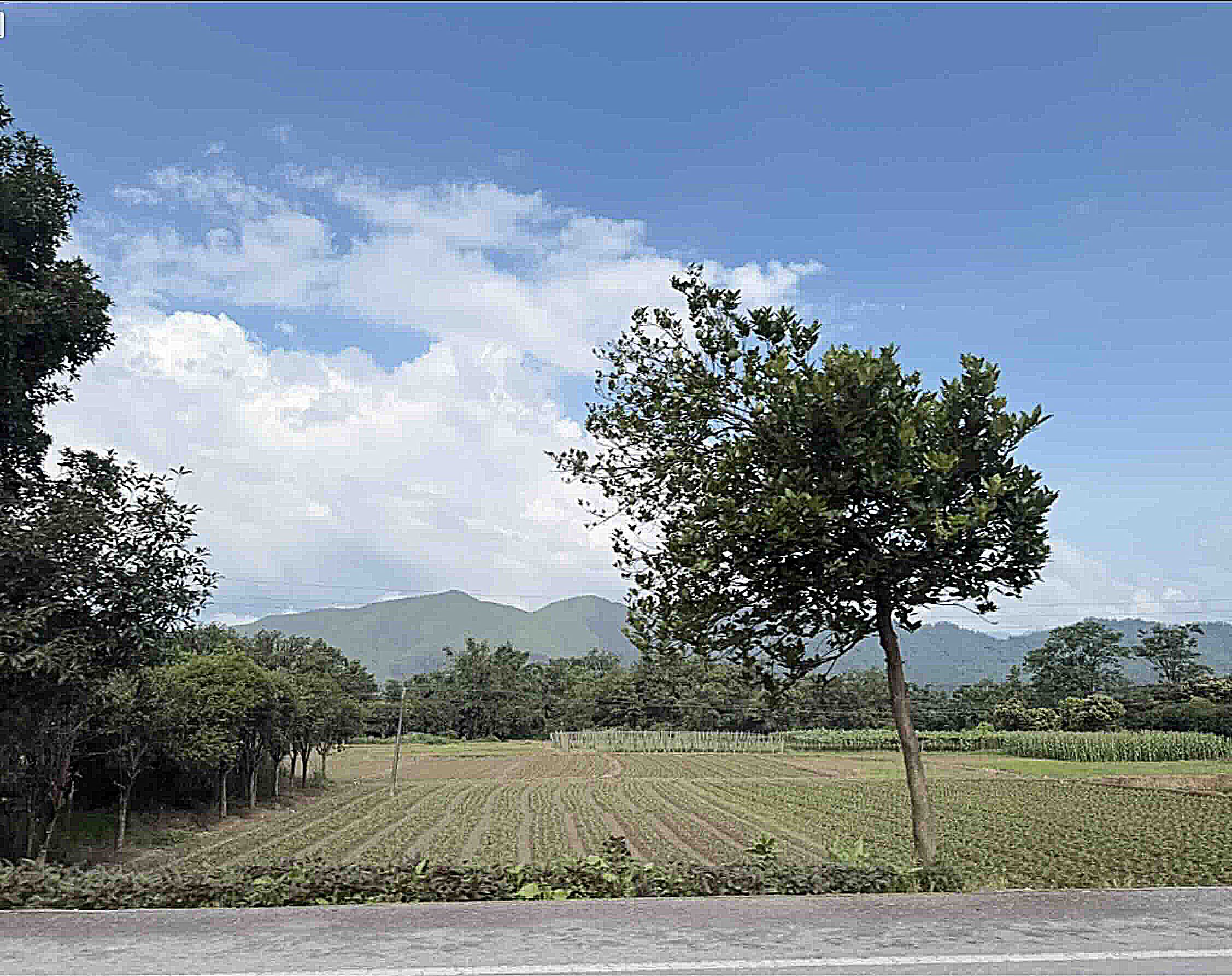
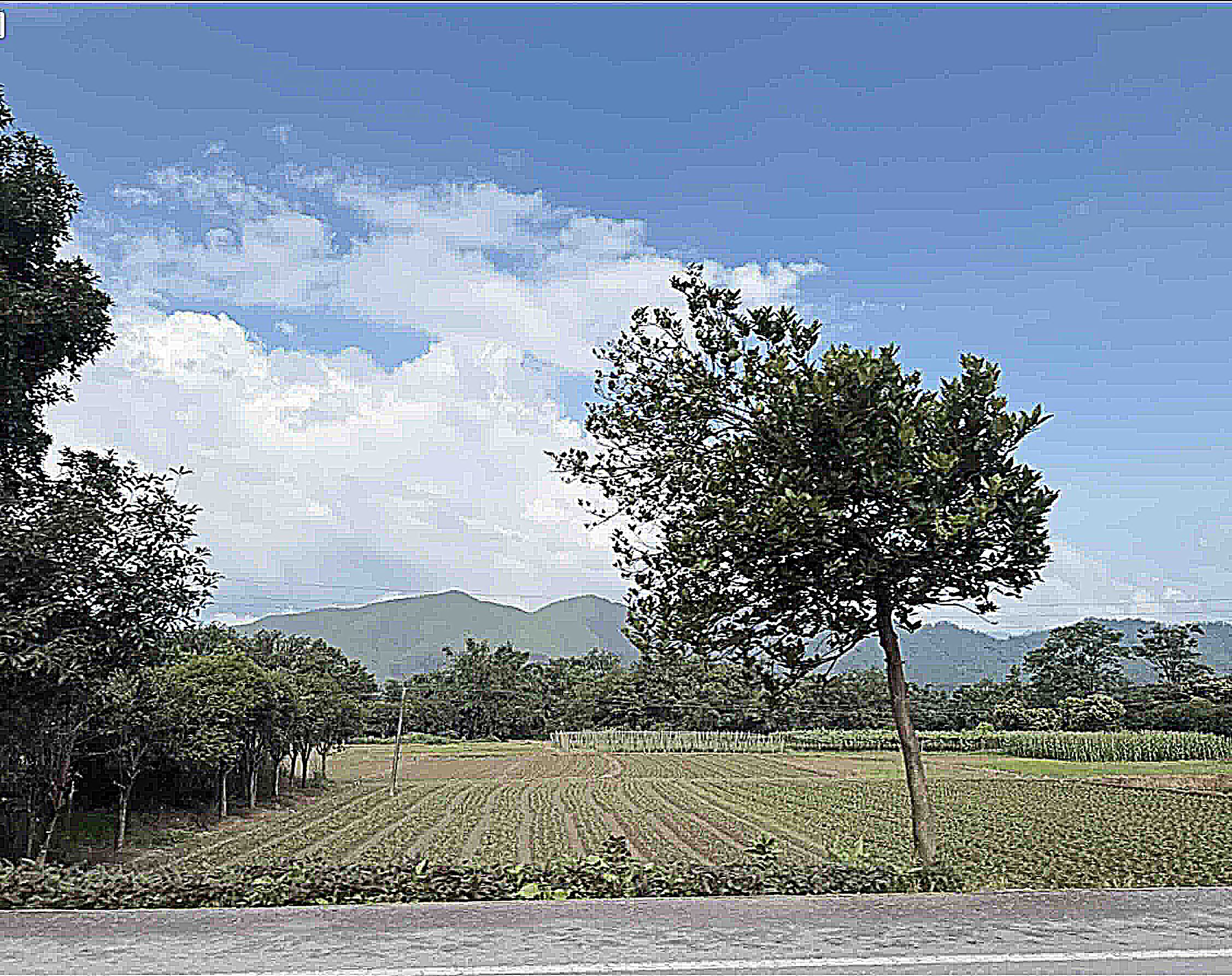
Guilin, China
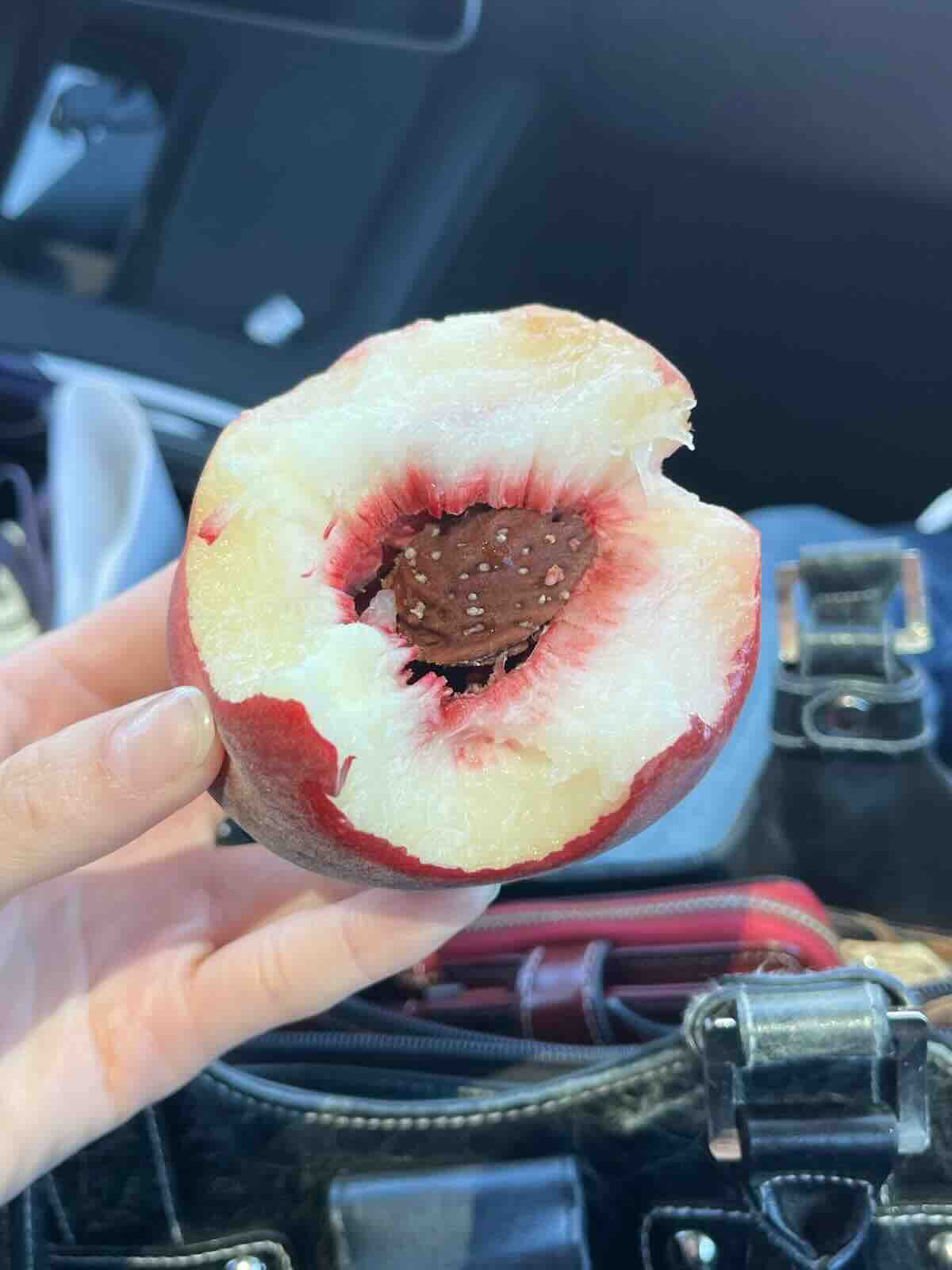
Peach from Oregon
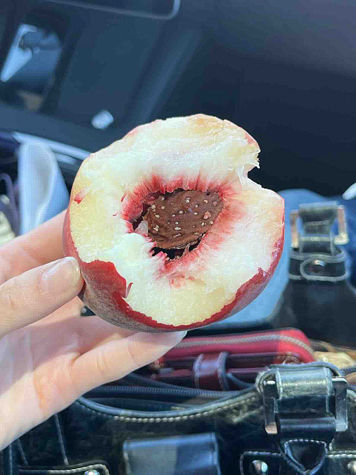
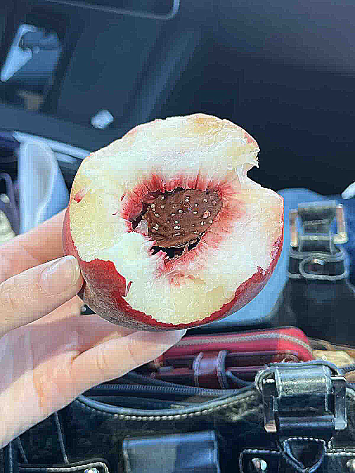
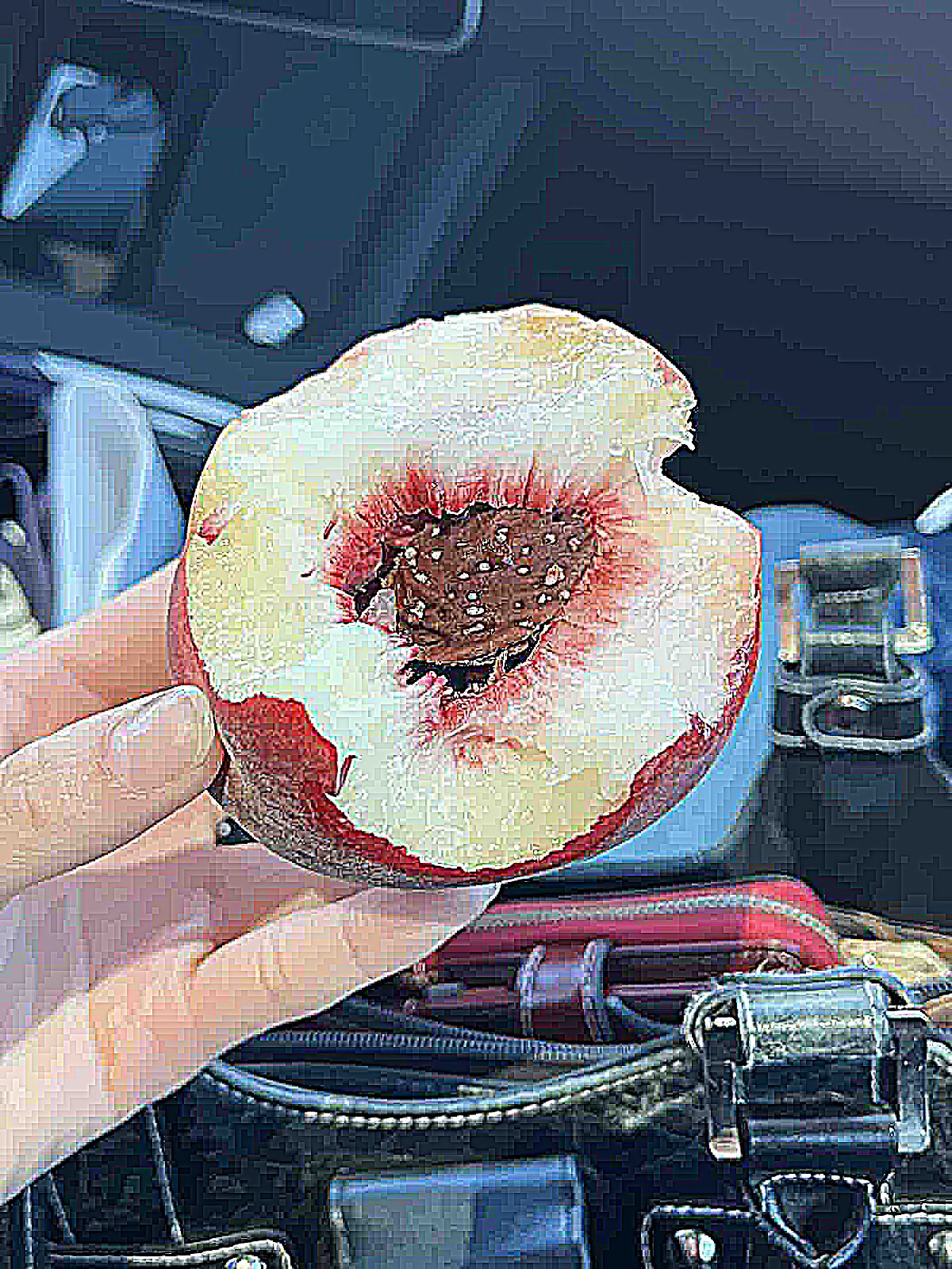
Experiment: Sharpen an Image, Blur It, then Sharpen It Again
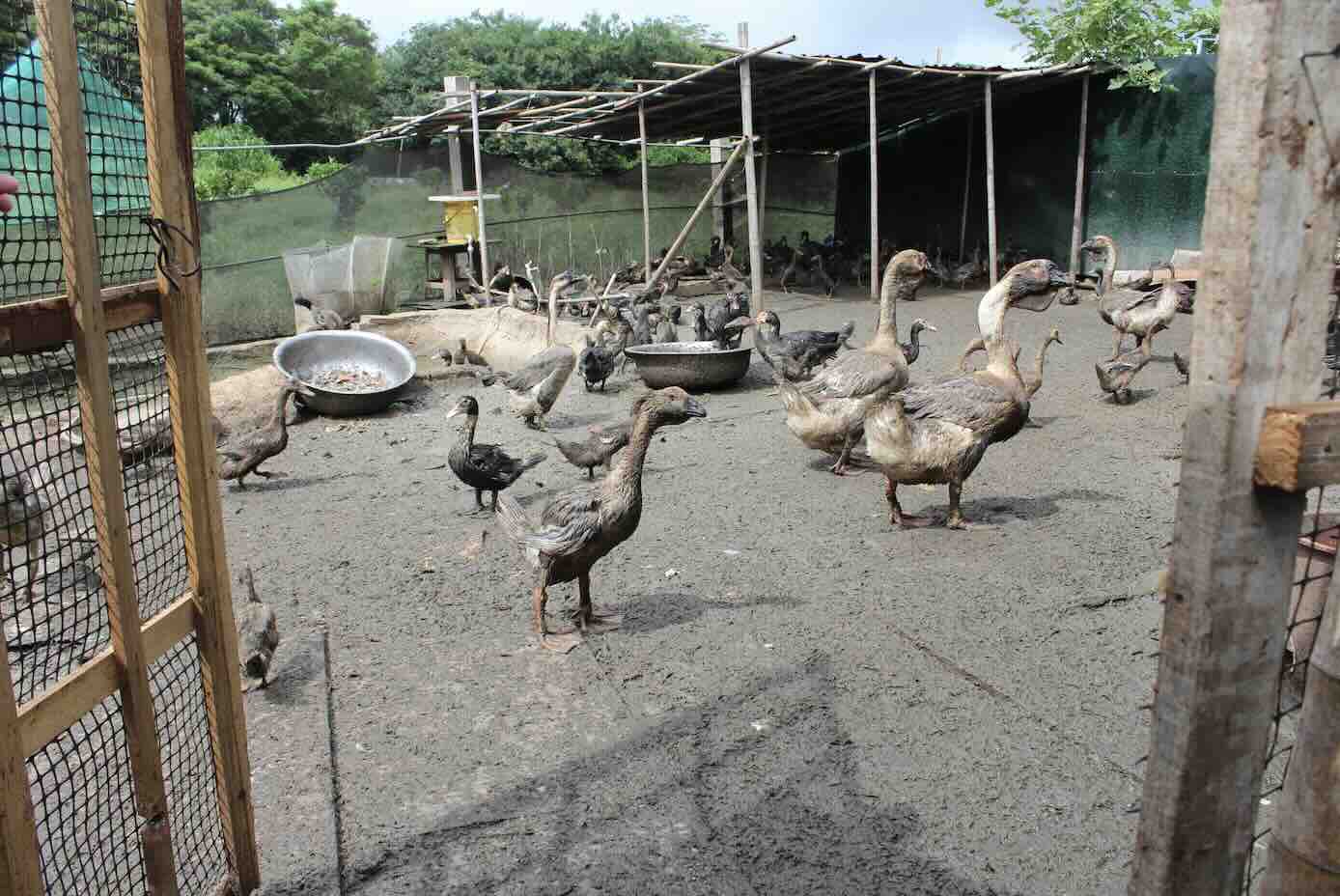
Ducks and geese in Dongshan, China
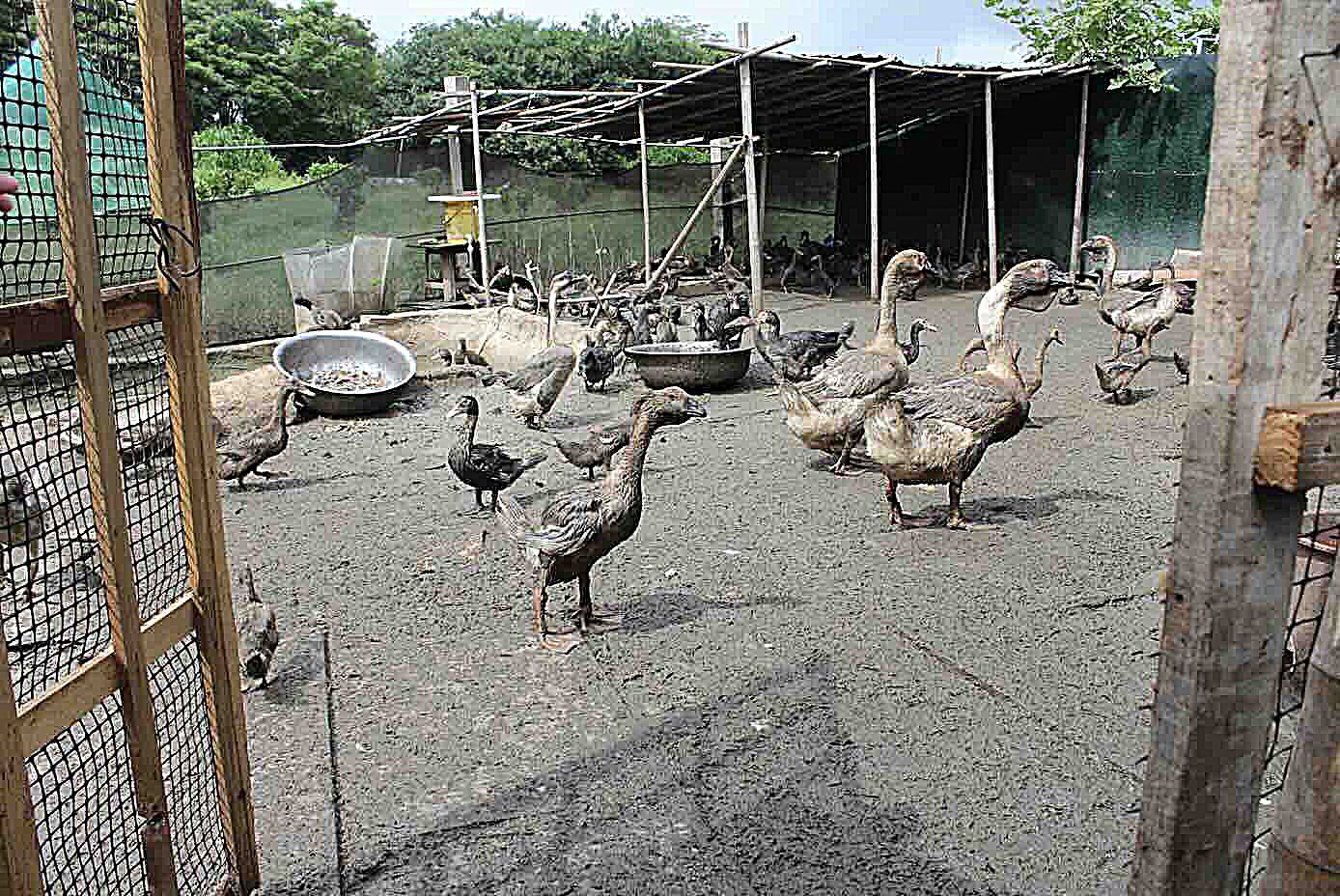
Sharpened ()
Sharpened → Blurred
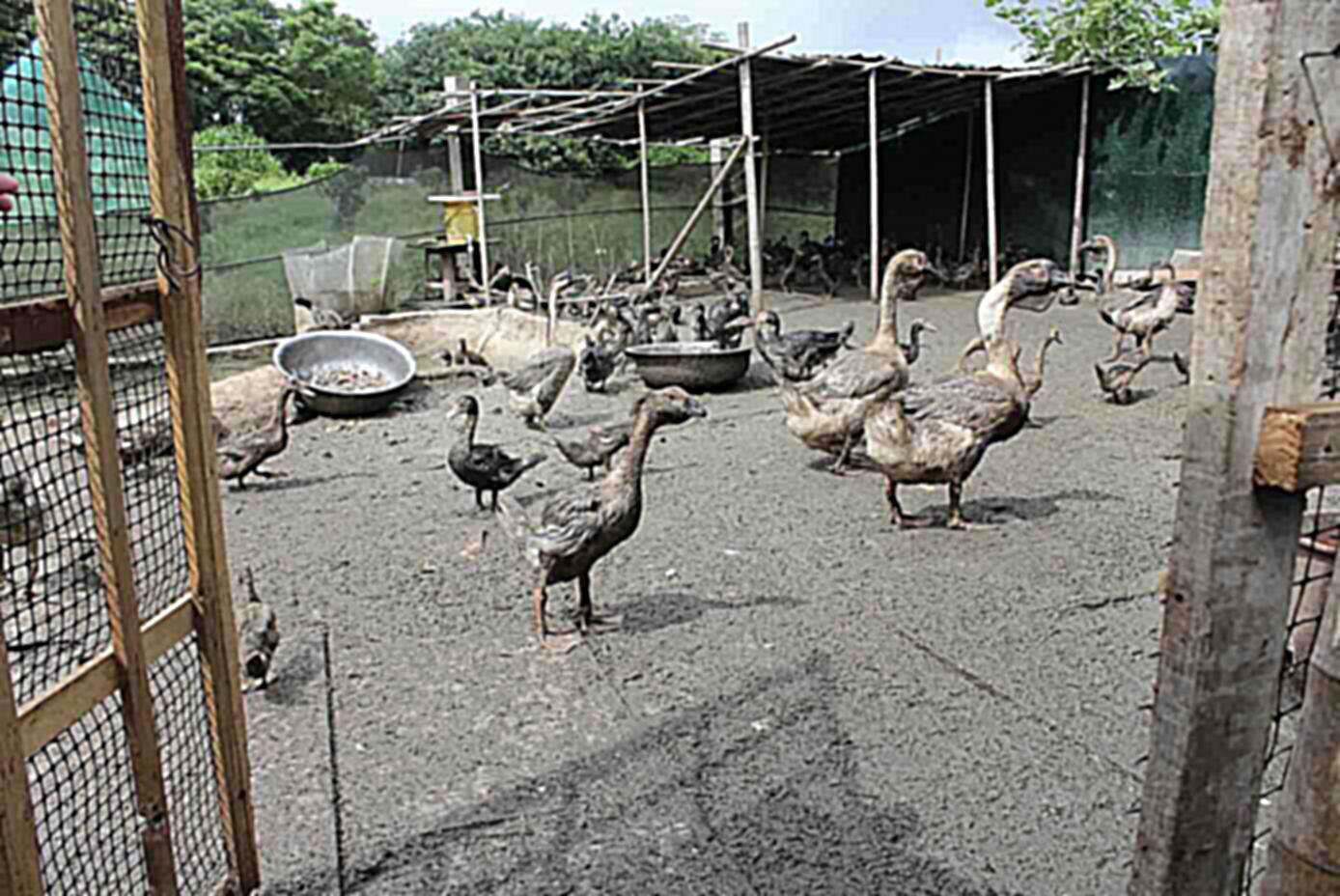
Sharpened → Blurred → Sharpened
* Looks less sharp compared to original and to first sharpening
Hybrid Images
2.2
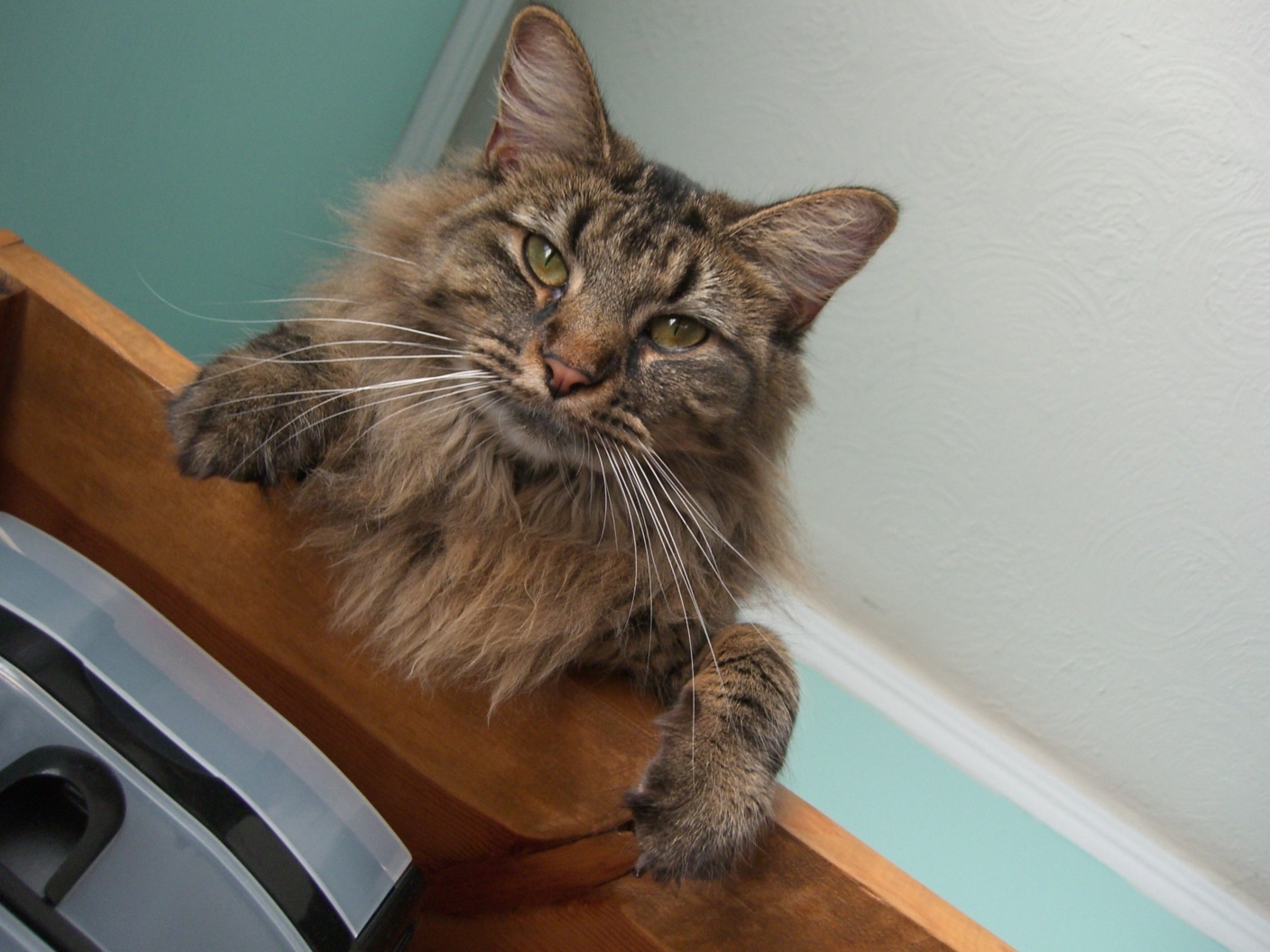
Nutmeg

Derek
Nutmeg and Derek Hybrid (BW-BW)
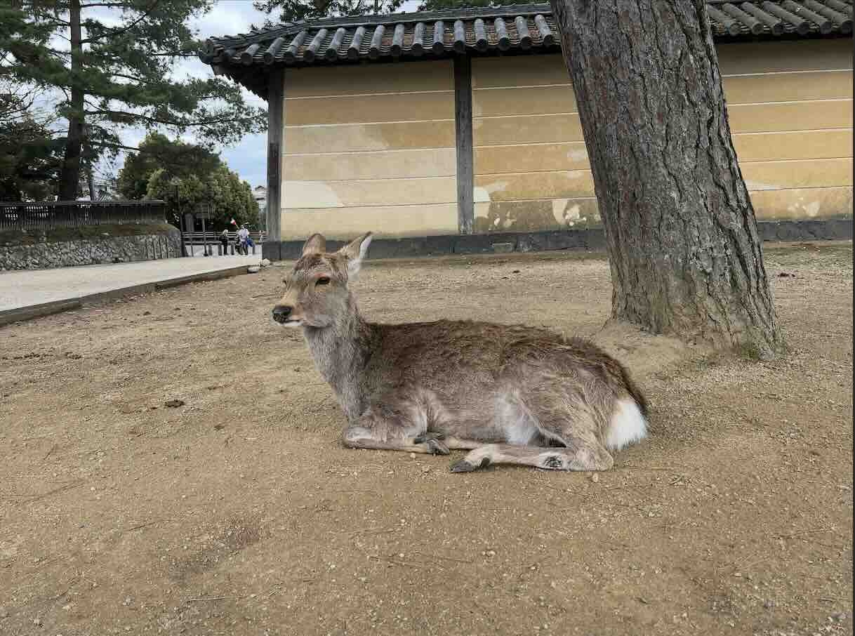
Nara, Japan Deer
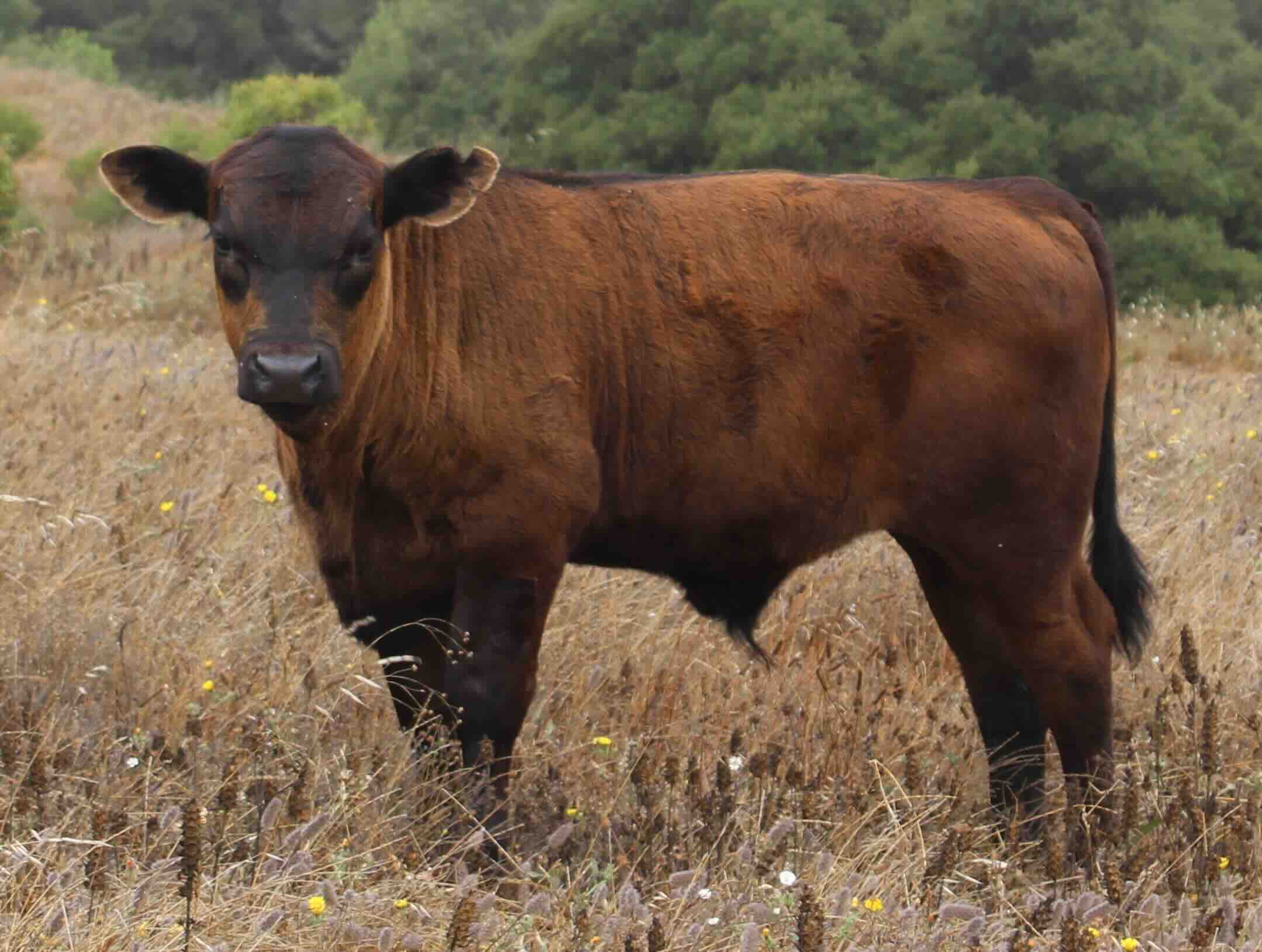
Tilden, Berkeley Cow
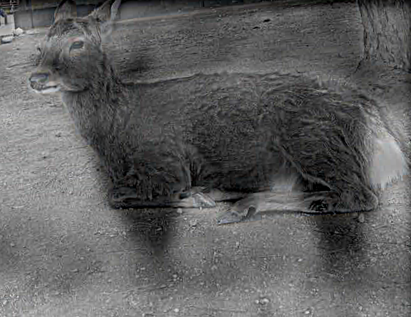
Nara, Japan Deer and Tilden, Berkeley Cow Hybrid (BW-BW)
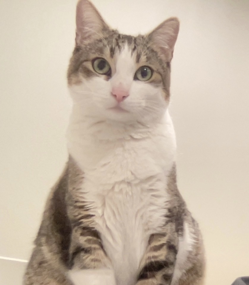
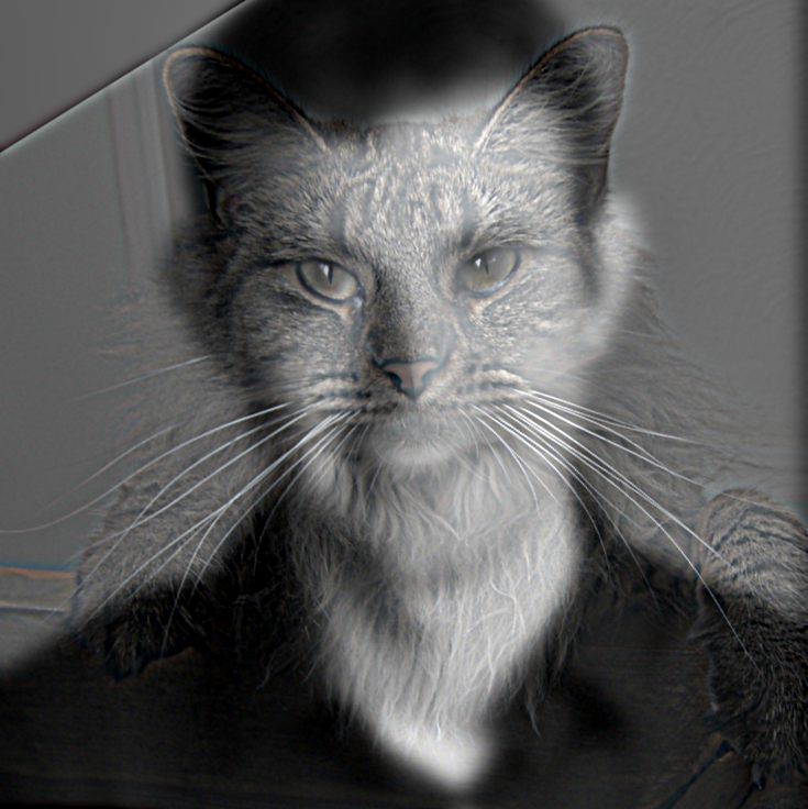
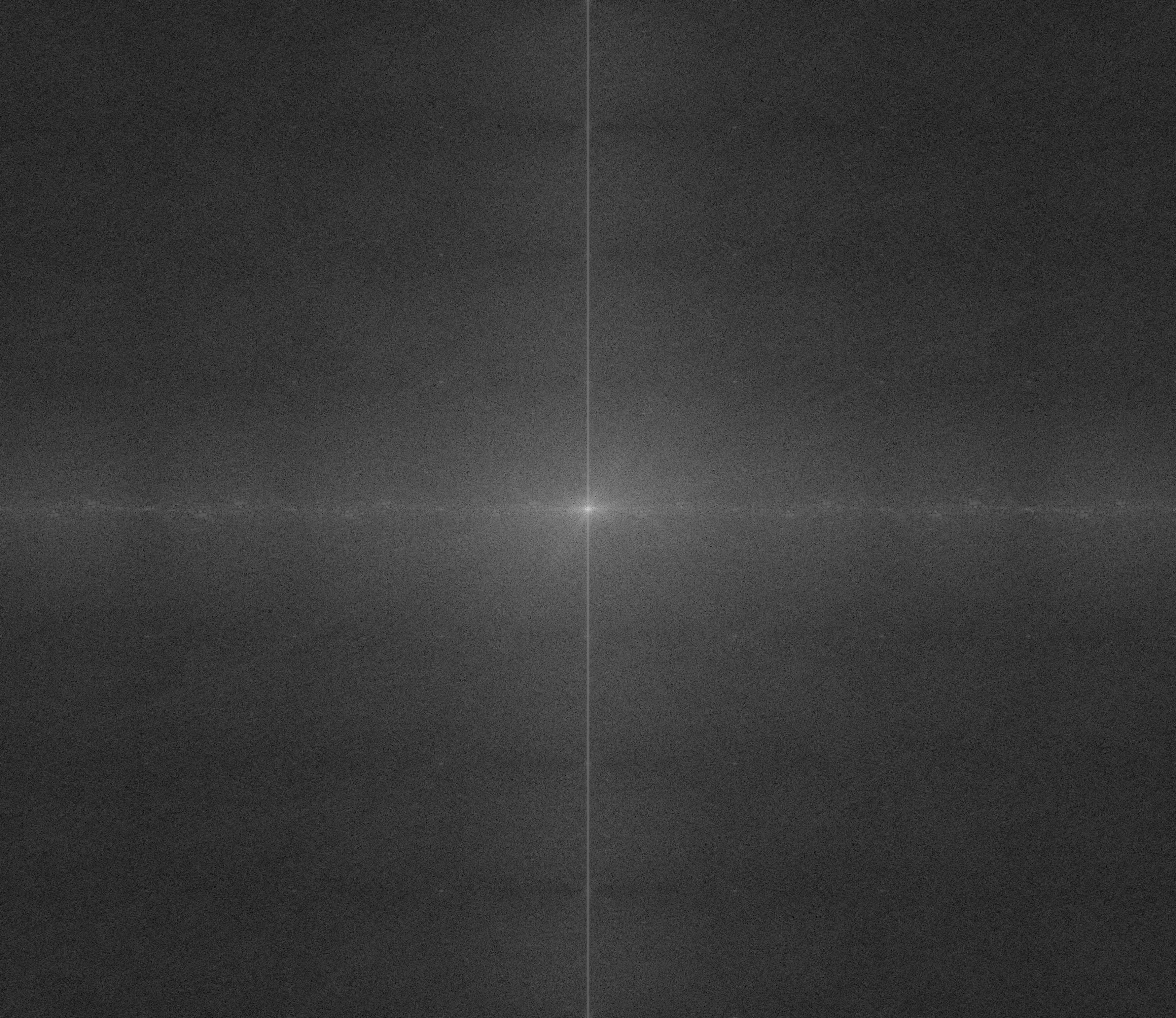
Carlos (my cat)
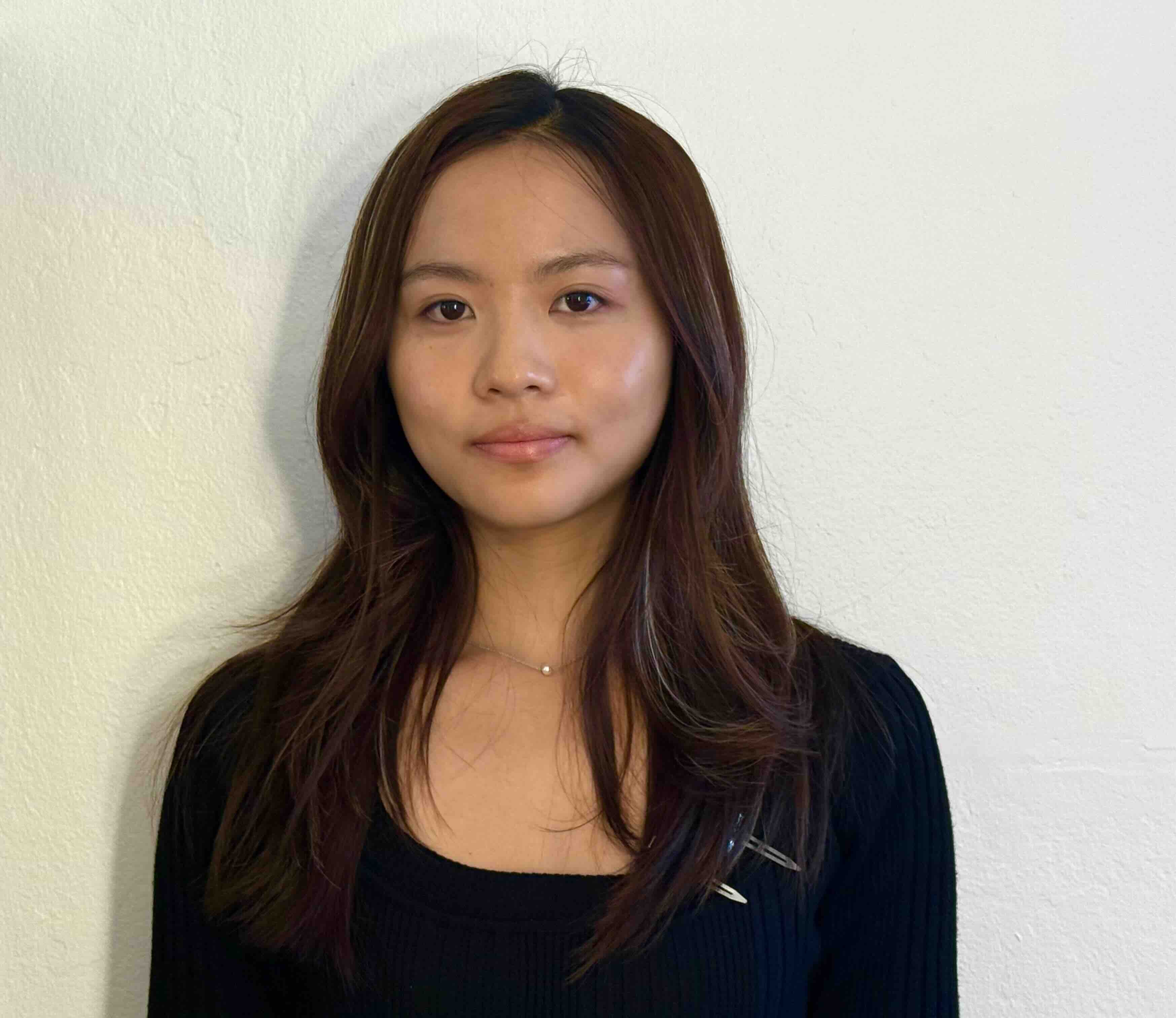
Self-portrait
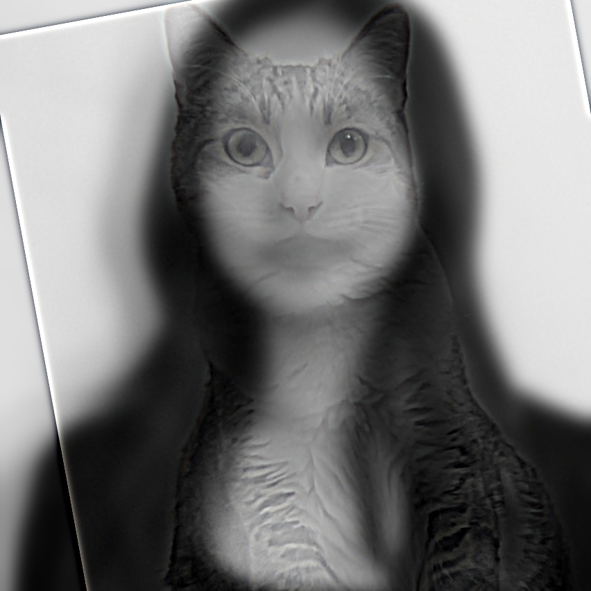
Carlos and Iana Self-Portrait Hybrid (BW-BW)
Carlos (my cat)
Self-portrait
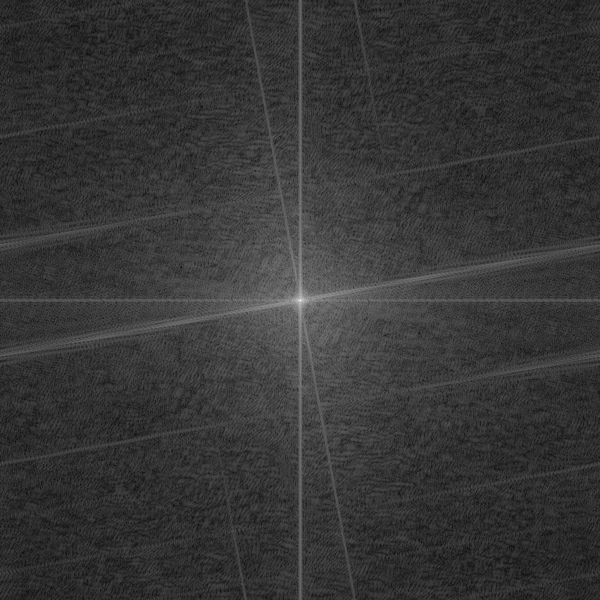
Carlos and Iana Self-Portrait Hybrid (BW-BW)
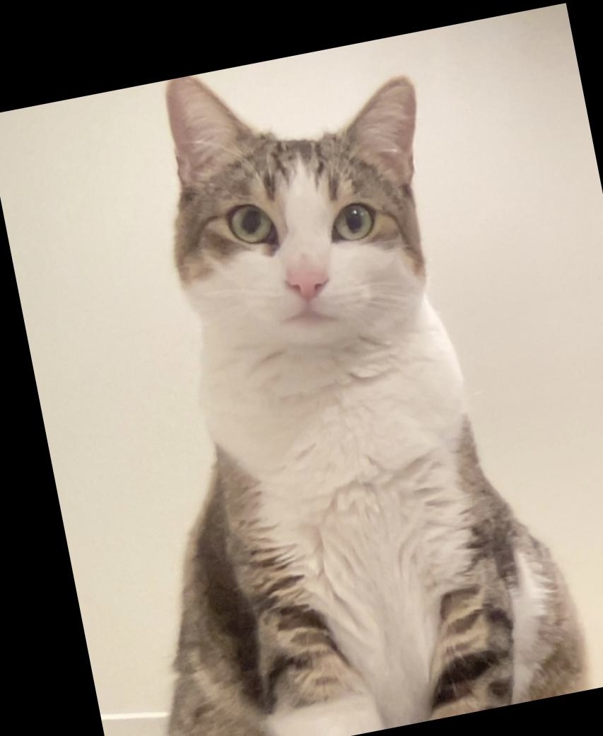
Carlos Aligned ()
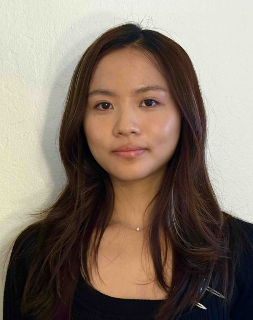
Self-portrait Aligned ()
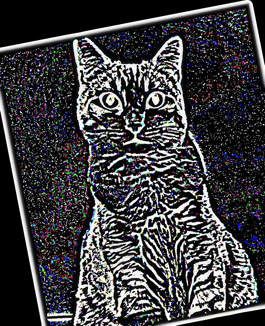
High Frequency Component
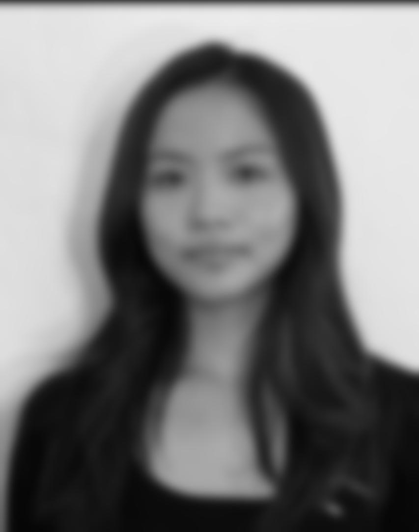
Low Frequency Component
I found that the output hybrid image seems to look better when using color only for the high-frequency component, and grayscale for the low-frequency component
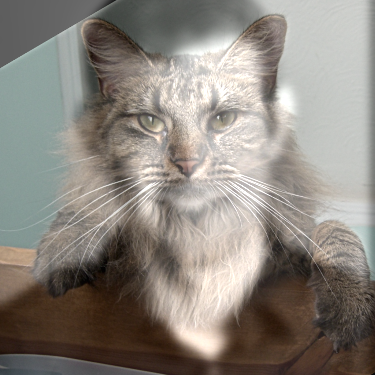
Nutmeg and Derek Hybrid (RGB-BW)
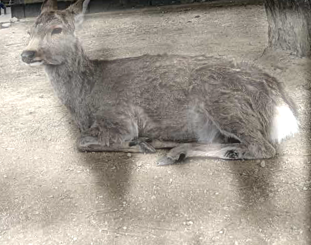
Nara, Japan Deer and Tilden, Berkeley Cow Hybrid (RGB-BW)
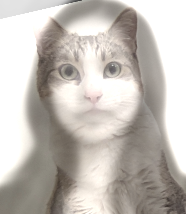
Carlos and Iana Self-Portrait Hybrid (RGB-BW)
Gaussian and Laplacian Stacks
2.3
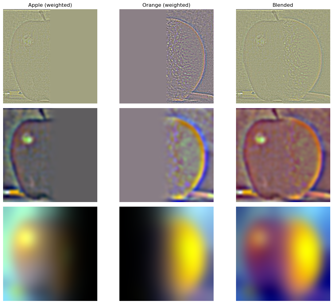
Recreation of Figure 3.42 in Szelski
2.4 Multiresolution Blending (a.k.a. the oraple!)
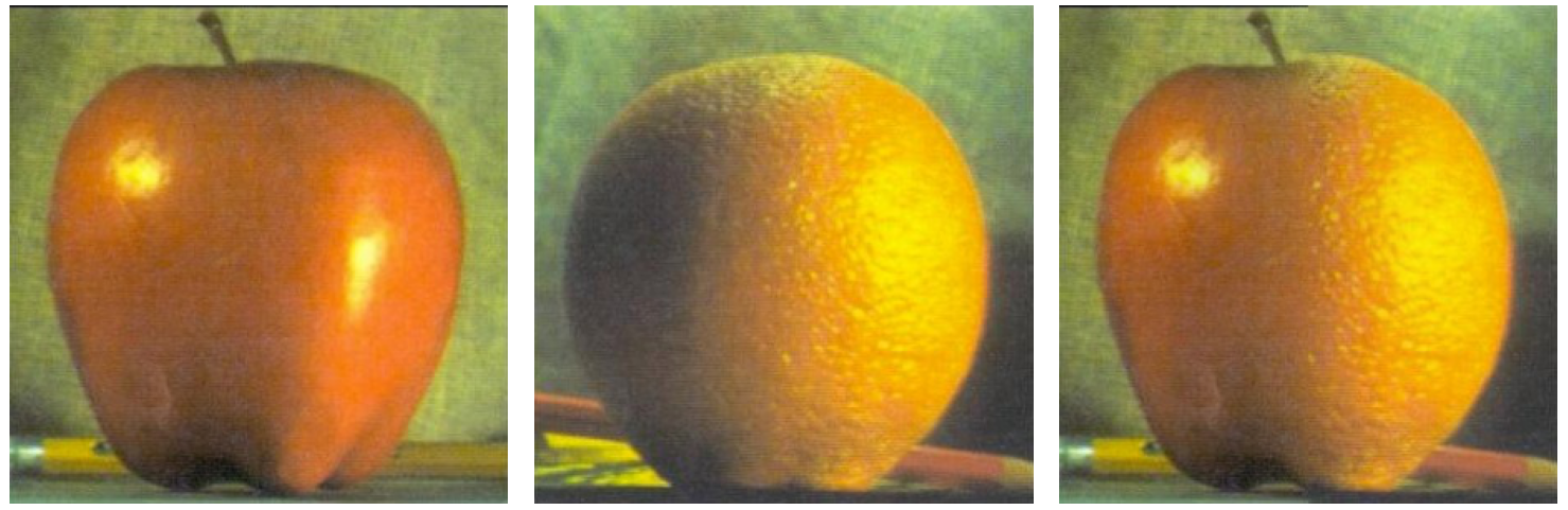
Oraple (vertical seam mask)
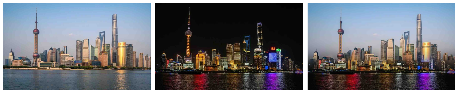
Shanghai -- Day and Night (horizontal seam mask)
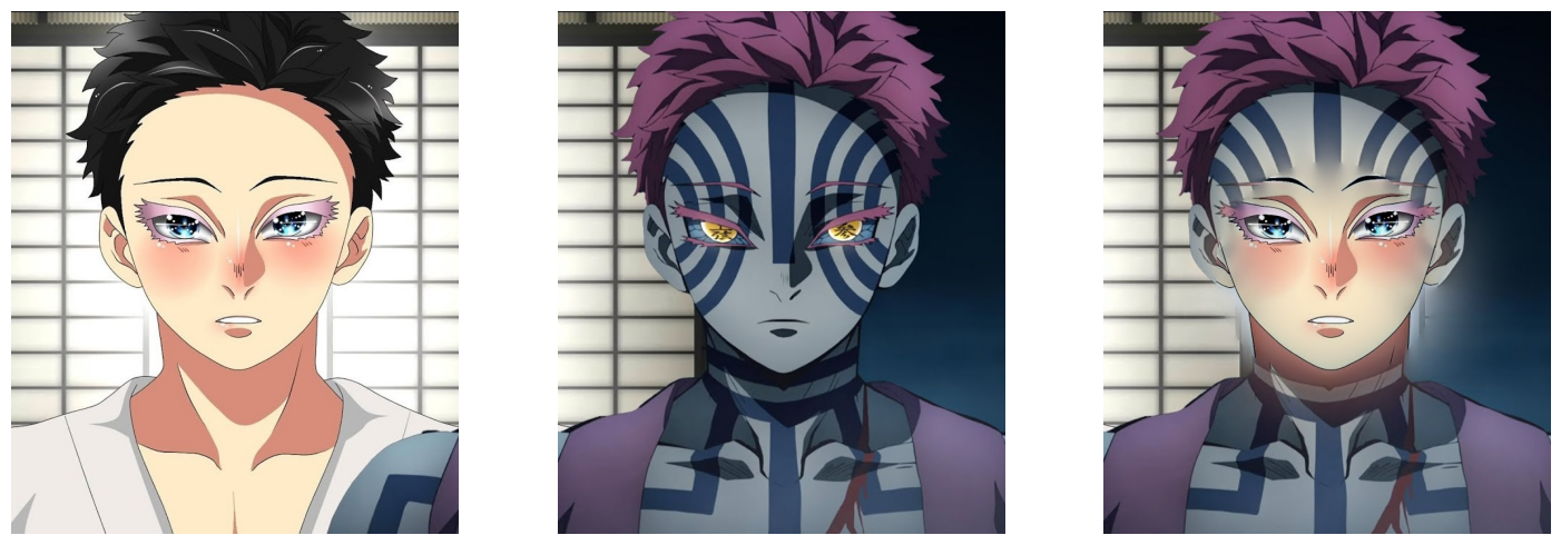
Akaza -- Before and After (circular mask)