Iana Lin — living systems

Overview

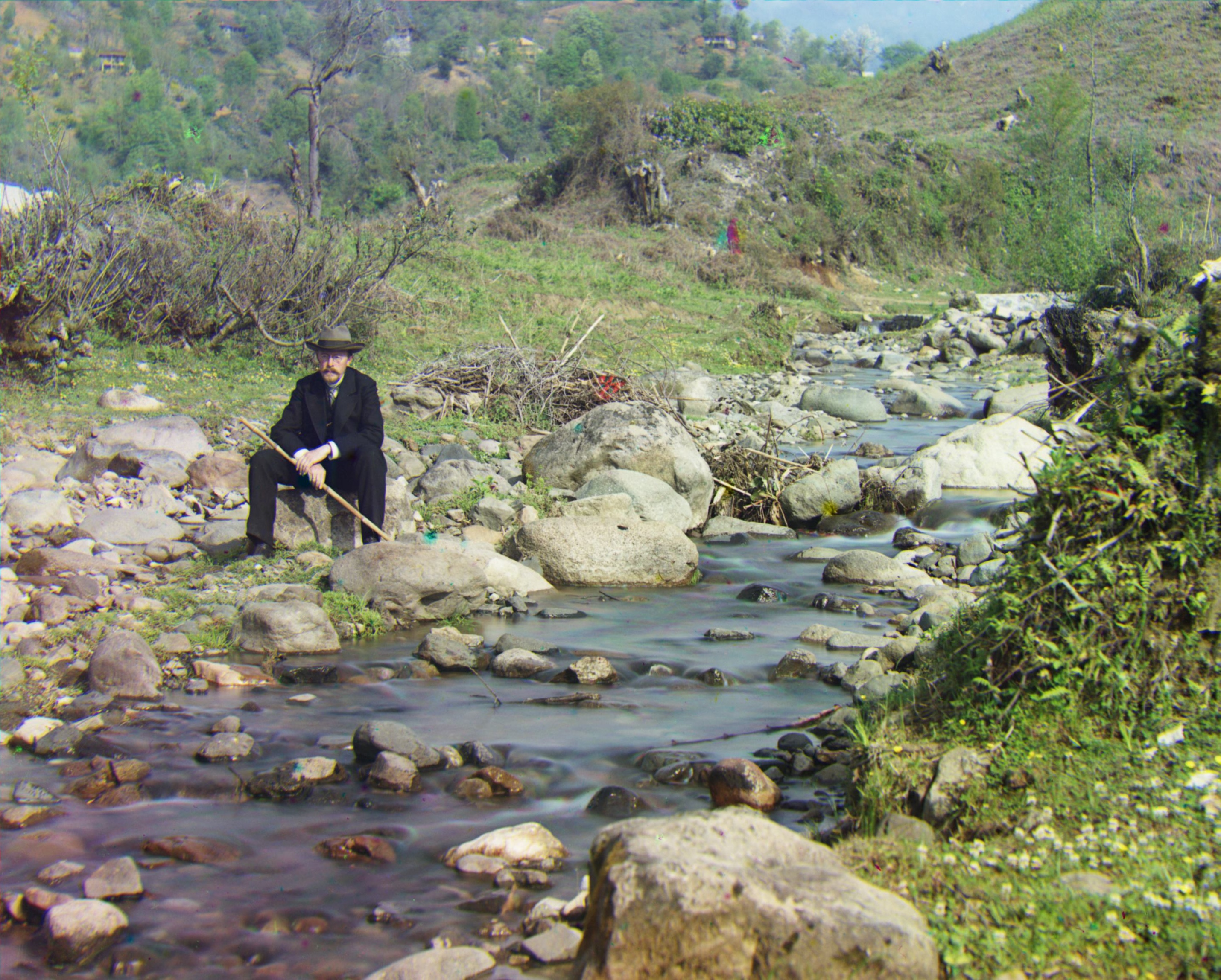
Self-portrait of Sergey Mikhaylovich Prokudin-Gorksii

Sergey Mikhaylovich Prokudin-Gorksii was a Russian chemist and photographer who pioneered colour photography in the early 20th-century. Prokudin-Gorskii created his negatives by exposing a glass plate of his unique camera three times in rapid succession, each with a different color filters: blue, green, and red. He then created positive glass slides of these negatives and projected them on top of each other.

The goal of this assignment is to automatically produce a color image by processing the digitized Prokudin-Gorksii glass plate images.

In order to do this, we will extract the three color channel images, align two of the channels to a reference channel (e.g. the blue channel), and then stack the together in the order of [r, g, b] to create a colored image. The question is...

How do we align two images effectively and efficiently?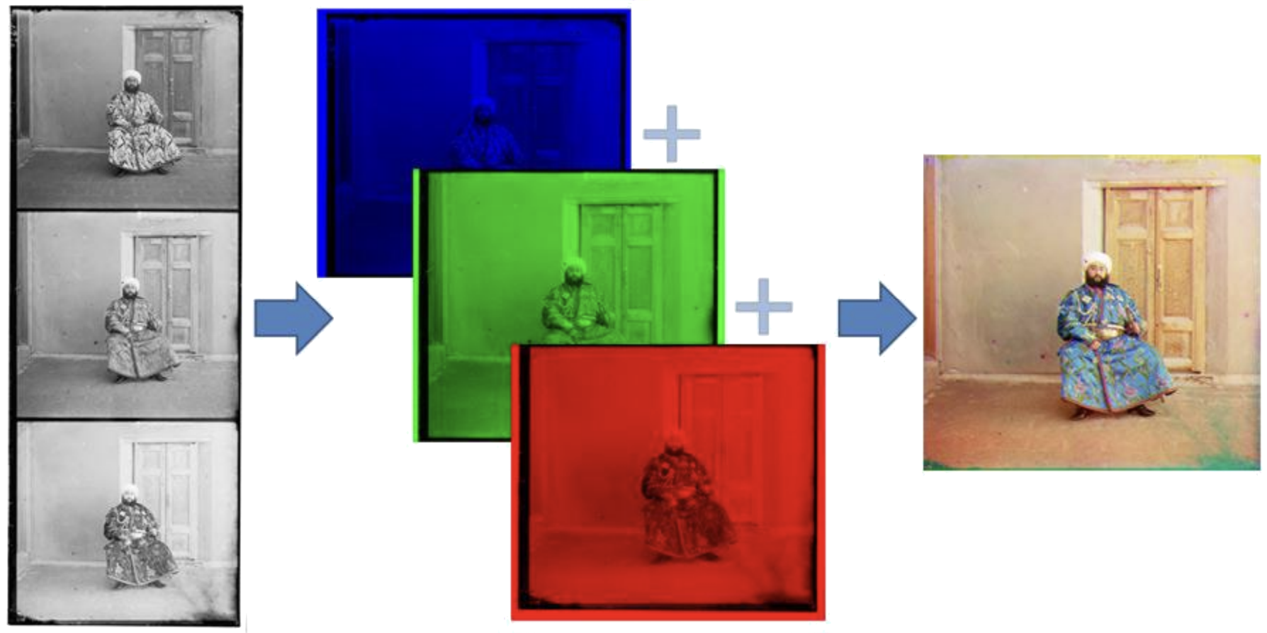

Image Alignment Schematic

Quantifying Image Alignment

Our goal can be formulated as an optimization problem where we seek to find the transformation parameters that maximize a certain objective function that measures the alignment between two images.

Alignment = f({Im}_A, {Im}_B)

Sum of Squared Differences / $l_2$ norm

A simple approach is to use:

f_{SSD}({Im}_A, {Im}_B) = -\left \Vert {Im}_A - {Im}_B \right \Vert_2 = -\sqrt{\sum\limits_{i} \sum\limits_{j} (A_{i,j}-B_{i,j})^2}

i.e. the negative

l_2

norm of the difference between the two images at each pixel. (We add a negative sign to the sum of squares so that we can maximize it instead of minimizing.)

However, this method measures the absolute difference between every pixel of the two images, making it sensitive to outliers (random bright/dark spots) and lighting changes between the two images.

Normalized Cross-Correlation (NCC)

A more robust approach is to use normalized cross-correlation, which measures the similarity between two images by comparing their intensity patterns.

f_{NCC}({Im}_A, {Im}_B) = \frac{1}{HW}\frac{\sum\limits_{i=1}^{H}\sum\limits_{j=1}^{W}\left((A_{i,j}-\bar{A})(B_{i,j}-\bar{B})\right)}{\sigma_A \sigma_B}

where

\bar{A}

and

\sigma_A

is the mean intensity of all pixels in A and their standard deviation, respectively.

H, W

are the height, width of the images.

This method is less sensitive to outliers and lighting changes, as it focuses on the relative pixel brightness differences between images rather than absolute values.

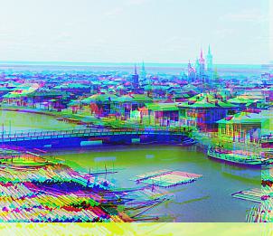
Image aligned with SSD Metric

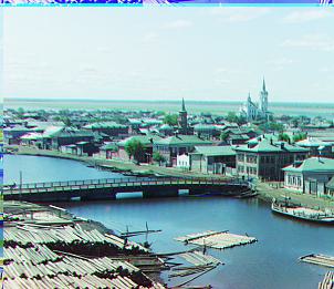
Image aligned with NCC Metric

Single-Scale Image Alignment

The naive alignment approach is to search every possible shift between two images. This method will give the alignment that maximizes the selected metric, based on the raw pixel brightness values.

Given that the three images Prokudin-Gorksii took at each scene were generally aligned, it is reasonable to search for best shift between a selected range [-displacement, displacement]. For each image's green and red channels, I tried every shift in both x and y directions within a [-15, 15] pixel range, choosing the shift that maximized the NCC metric with the blue channel.

Challenges with Border Artifacts

However, the NCC (as well as SSD) metric treats each pixel equally and every channel equally, which is not ideal. Due to the filming conditions and the filters obscuring light differently across channels, border regions often contain artifacts and noise that can mislead alignment algorithms. Additionally, the digitization process may introduce edge artifacts that don't represent the actual image content.

Since alignment metrics weight all pixels equally, these border pixels can affect the optimization, leading to suboptimal alignments. Cropping the borders focuses the alignment on the central, high-confidence image content, significantly improving results.

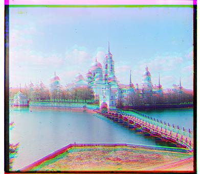
Image aligned without cropping

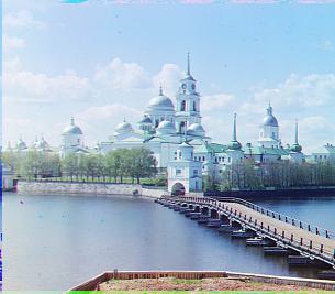
Image aligned after cropping 11% border pixels

Aligned Low-Resolution Images:

Note: offsets are in the form $(\Delta y, \Delta x)$

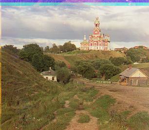
Cathedral
G: (5, 2)
R: (12, 3)

Monastery
G: (-3, 2)
R: (3, 2)

Tobolsk
G: (3, 3)
R: (6, 3)

However, this brute-force search is computationally expensive, especially for high-resolution images.

Multi-Scale Image Alignment

For high-resolution images, searching all possible shifts becomes computationally prohibitive because the optimal pixel displacement is usually be much larger. (Pixels become "smaller" or cover less visual space.) A multi-scale approach using image pyramids significantly reduces computational requirements

The algorithm works by

recursively downsampling the both the reference and current image by a factor of 2 (I chose to downsample 2-6 times for a total of 3-7 layers in the image pyramid)
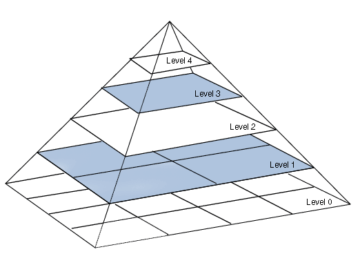
aligning the images at the coarsest scale (i.e. aligning the smallest images)
updating a total_offset variable and refining the alignment at progressively finer scales
offset = find_alignment(reference_level, current_level_aligned, search_range)

total_offset = (total_offset[0] + offset[0], total_offset[1] + offset[1])
# we need to double the offset at every level except for the last (finest level) because every image's resolution is doubled
total_offset = (total_offset[0] * 2, total_offset[1] * 2)

# we can shrink search range at every level
search_range = max(2, search_range // 2)

This reduces the search space from potentially hundreds or thousands of pixels at each level to a manageable range.

Performance Improvement:

~1.5 seconds per image vs ~5+ seconds with naive search, while achieving identical alignment results on low-resolution images.

Aligned High-Resolution Images:

Note: offsets are in the form $(\Delta y, \Delta x)$

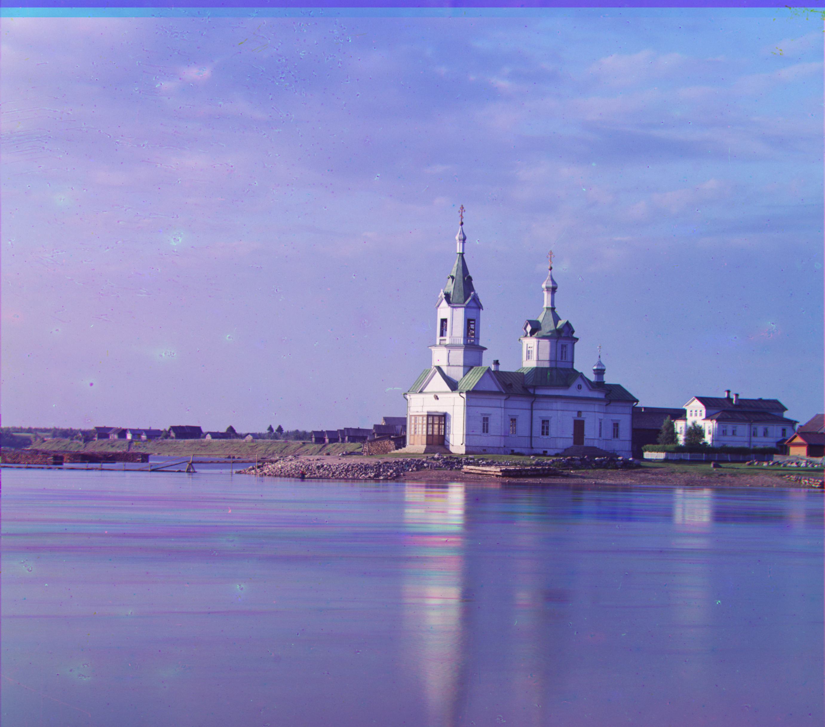
Church
G: (25, 4)
R: (58, -4)

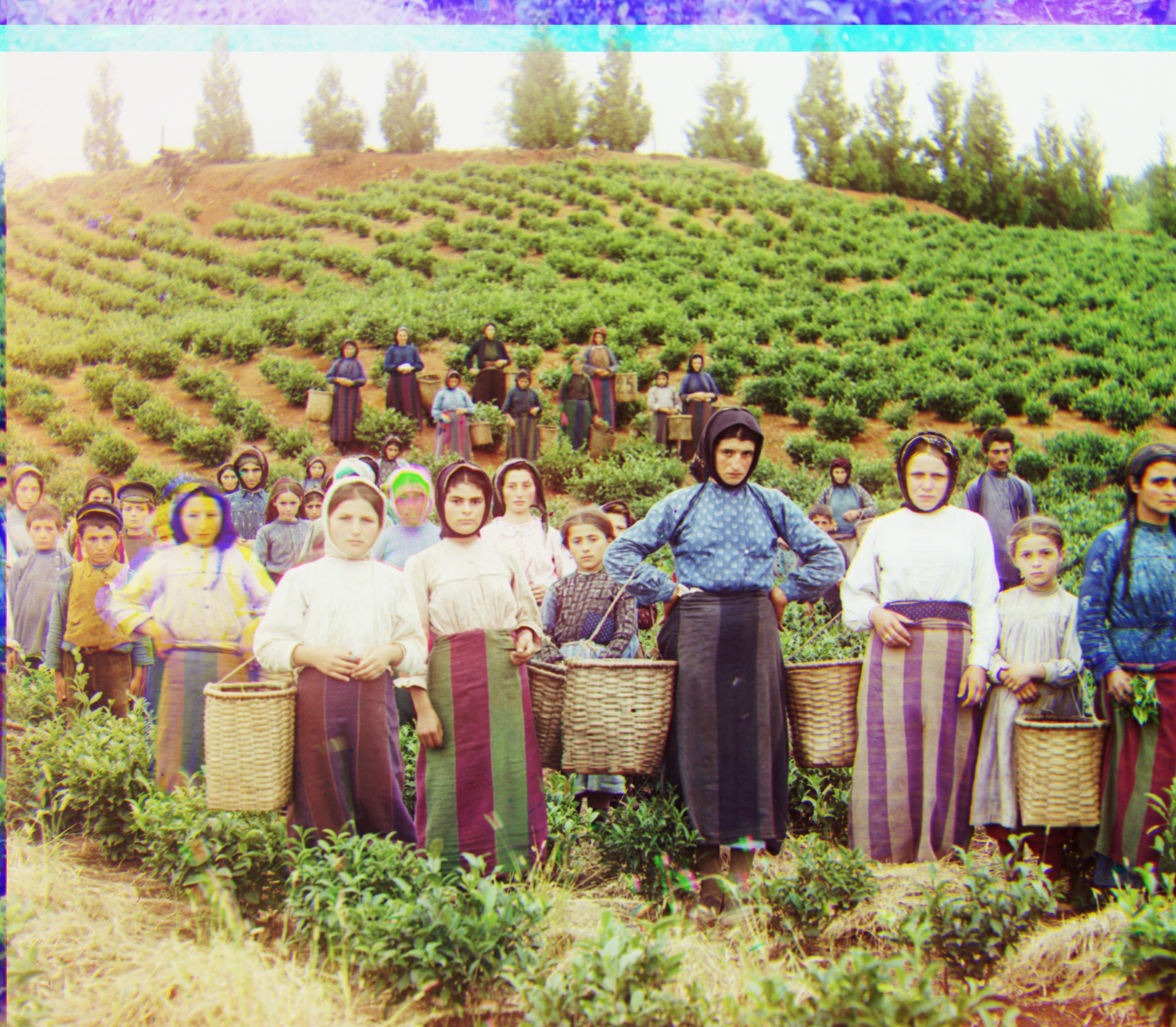
Harvesters
G: (59, 16)
R: (123, 13)

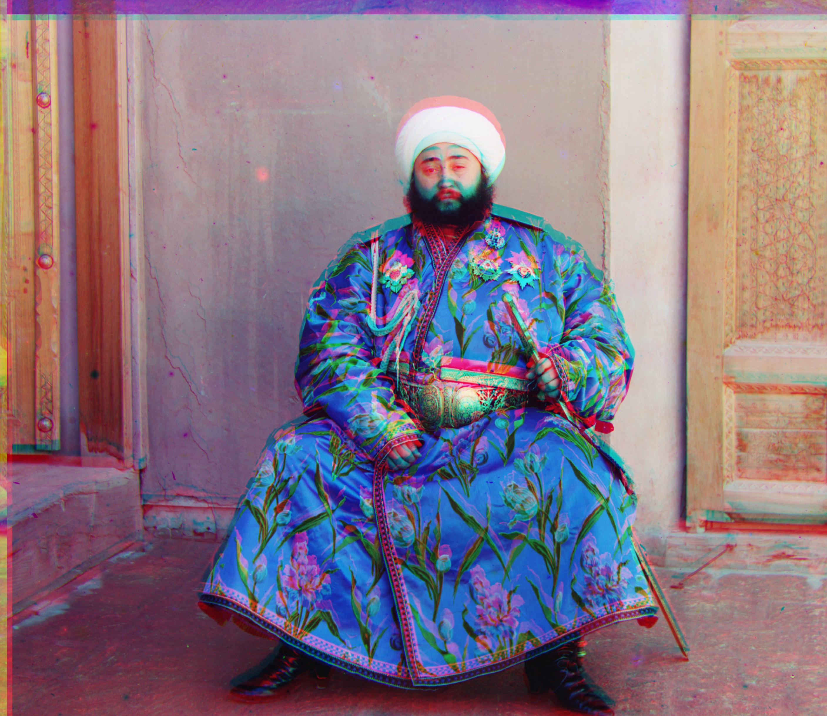
Emir
G: (49, 24)
R: (43, -989)*

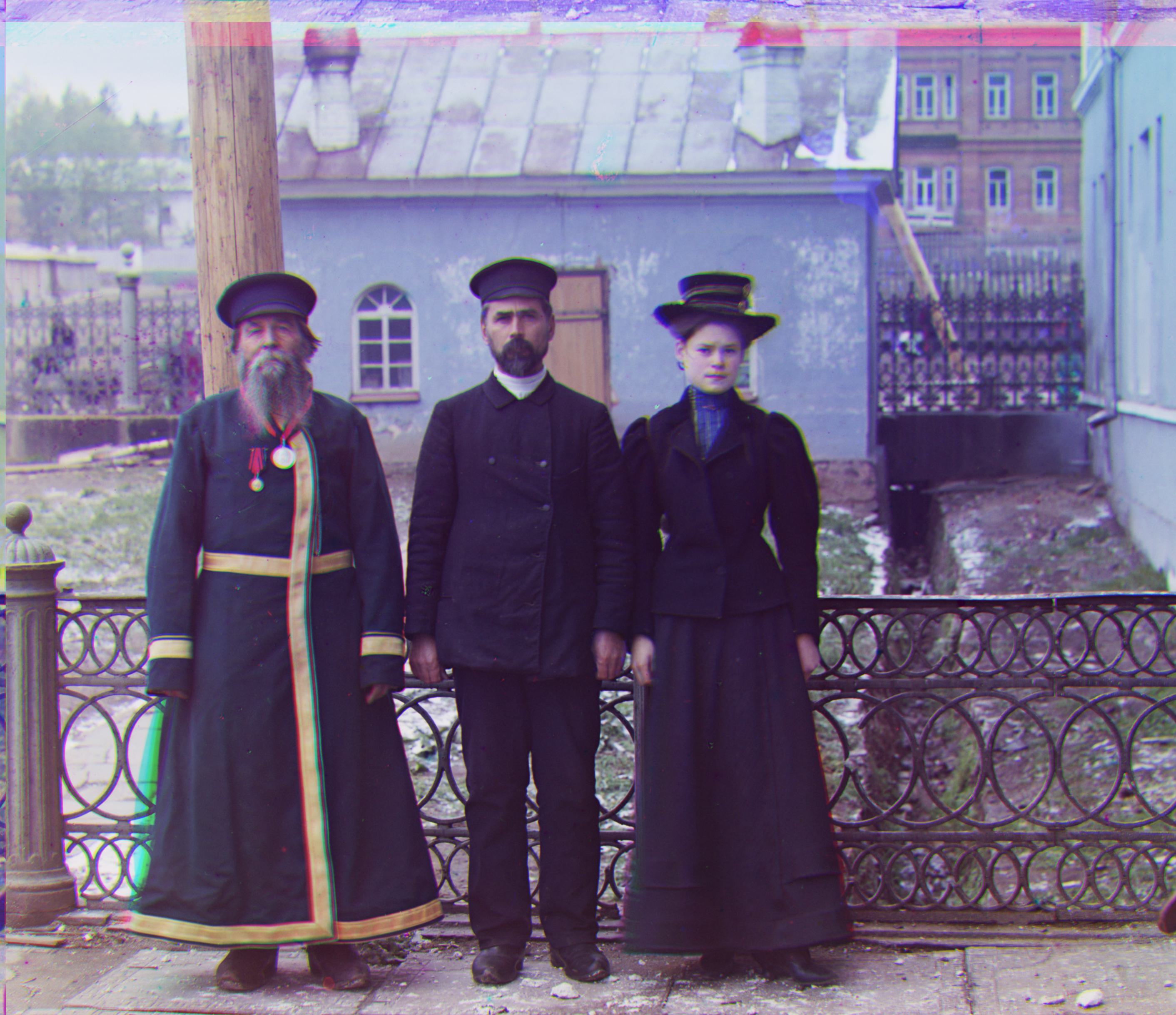
Three Generations
G: (53, 14)
R: (111, 11)

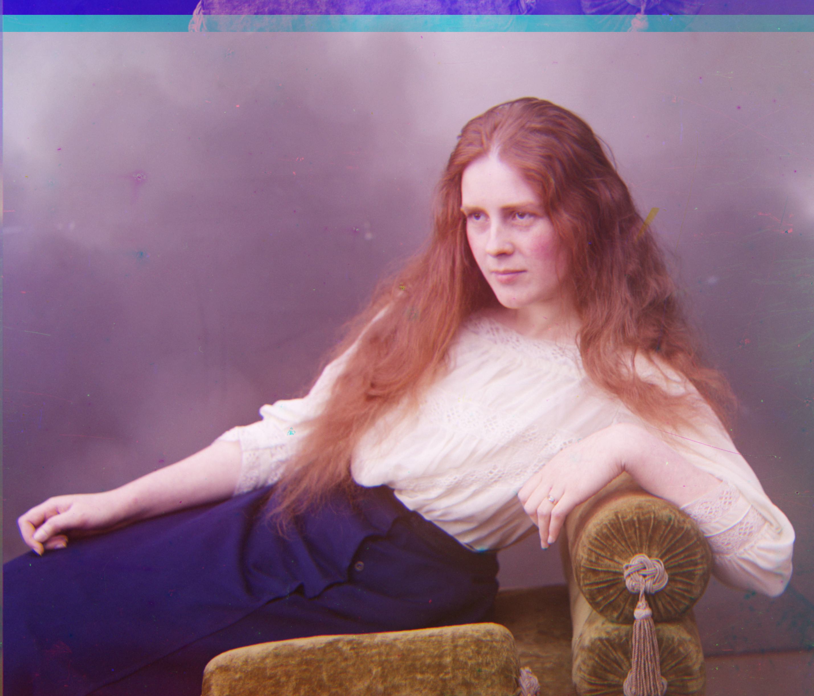
Lady
G: (52, 9)
R: (112, 12)

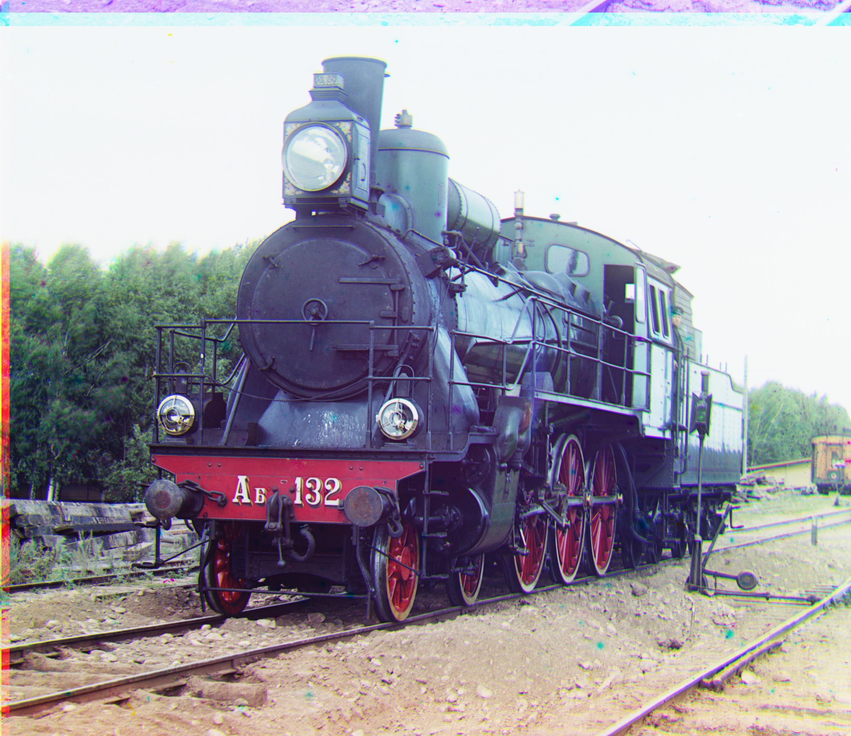
Train
G: (42, 5)
R: (87, 32)

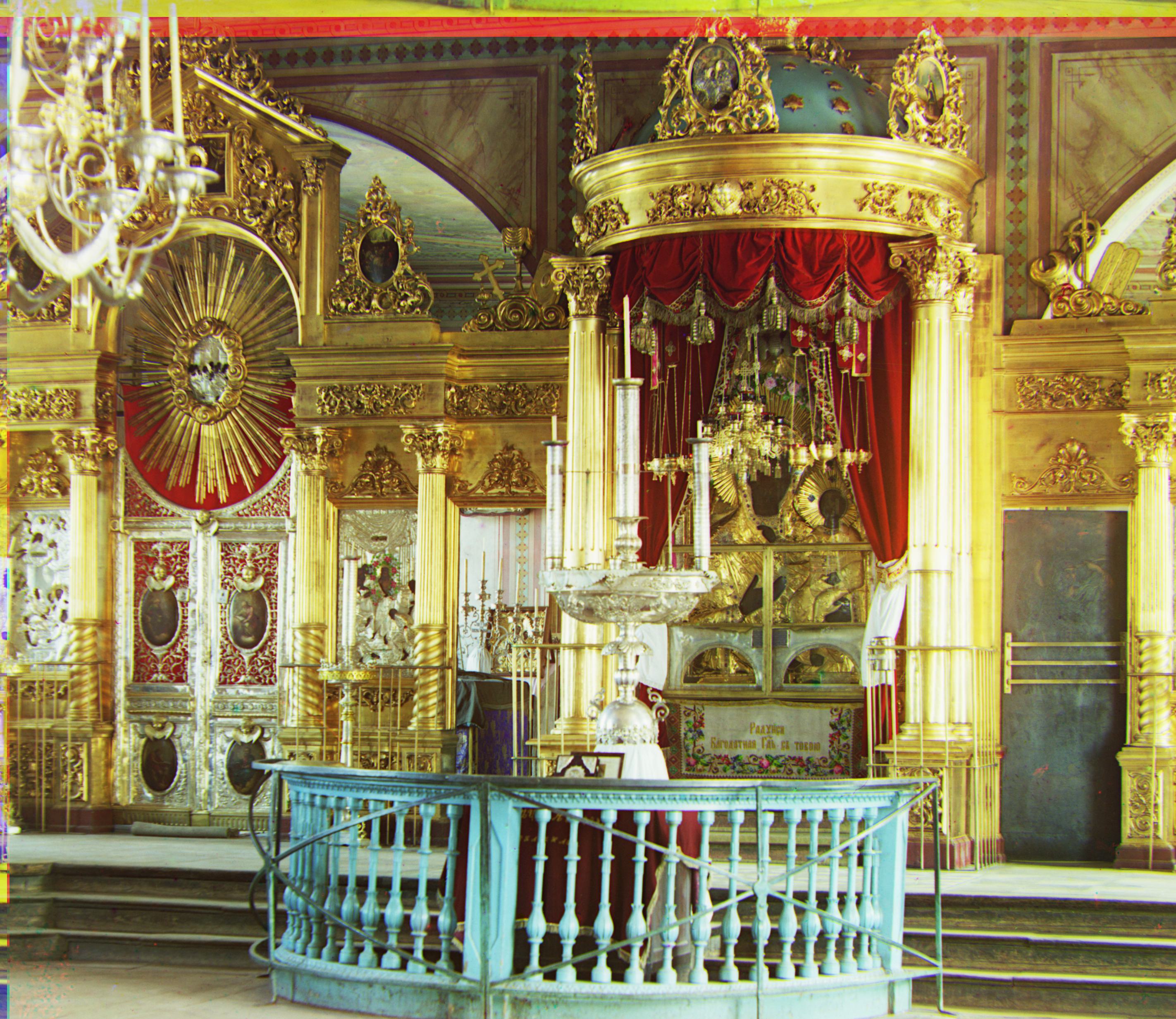
Icon
G: (41, 17)
R: (89, 23)

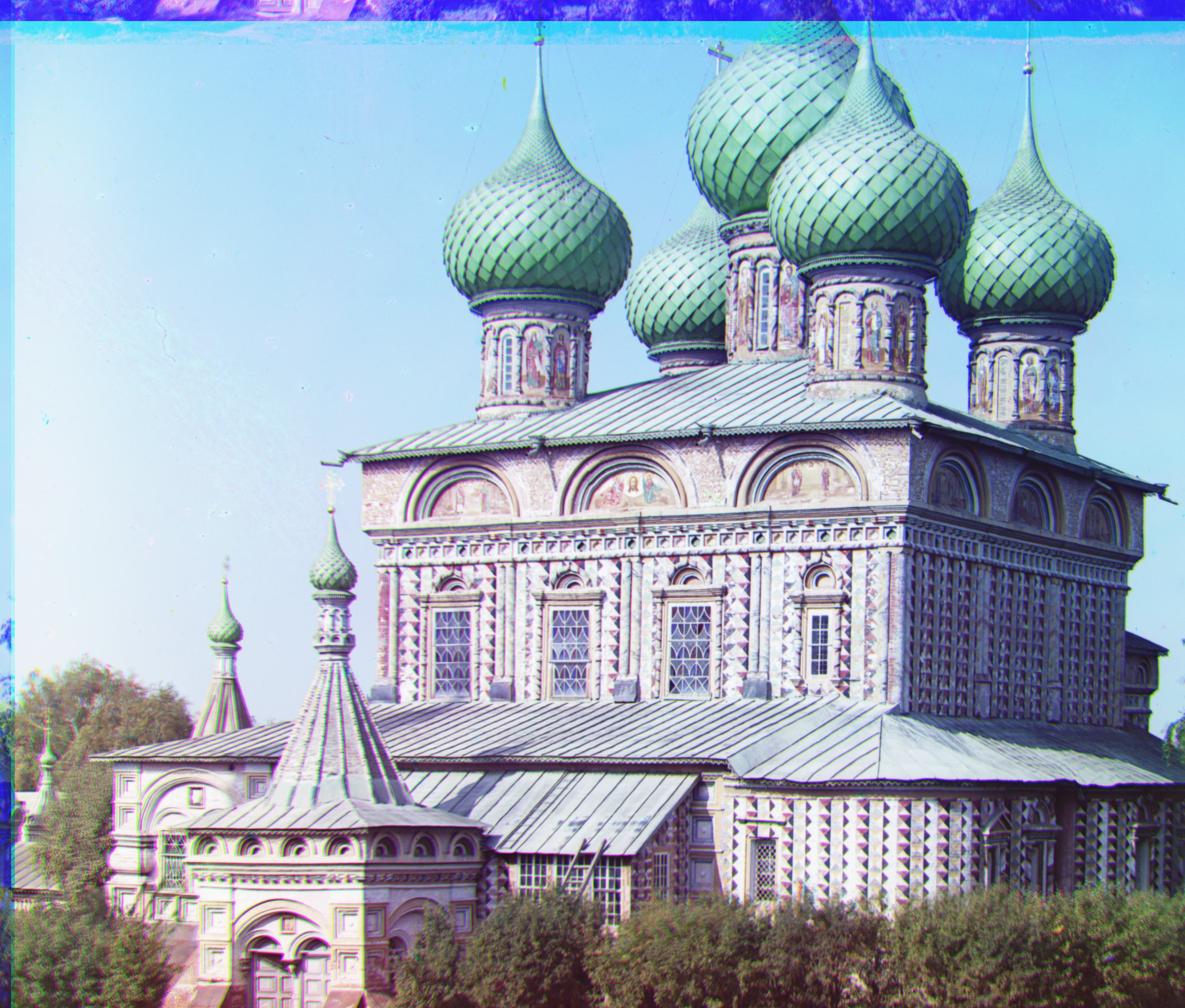
Onion Church
G: (51, 27)
R: (108, 36)

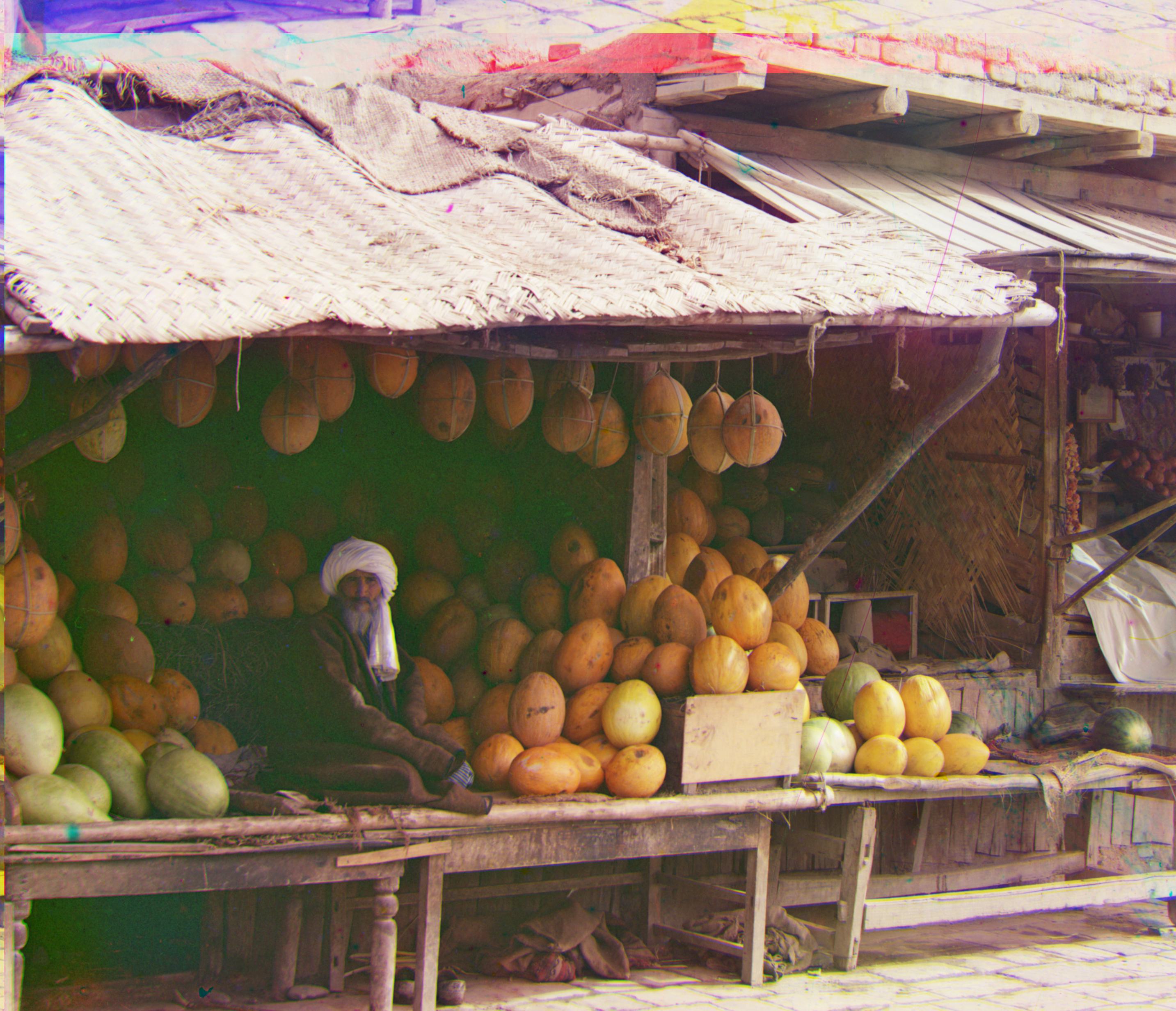
Melons
G: (81, 10)
R: (178, 13)

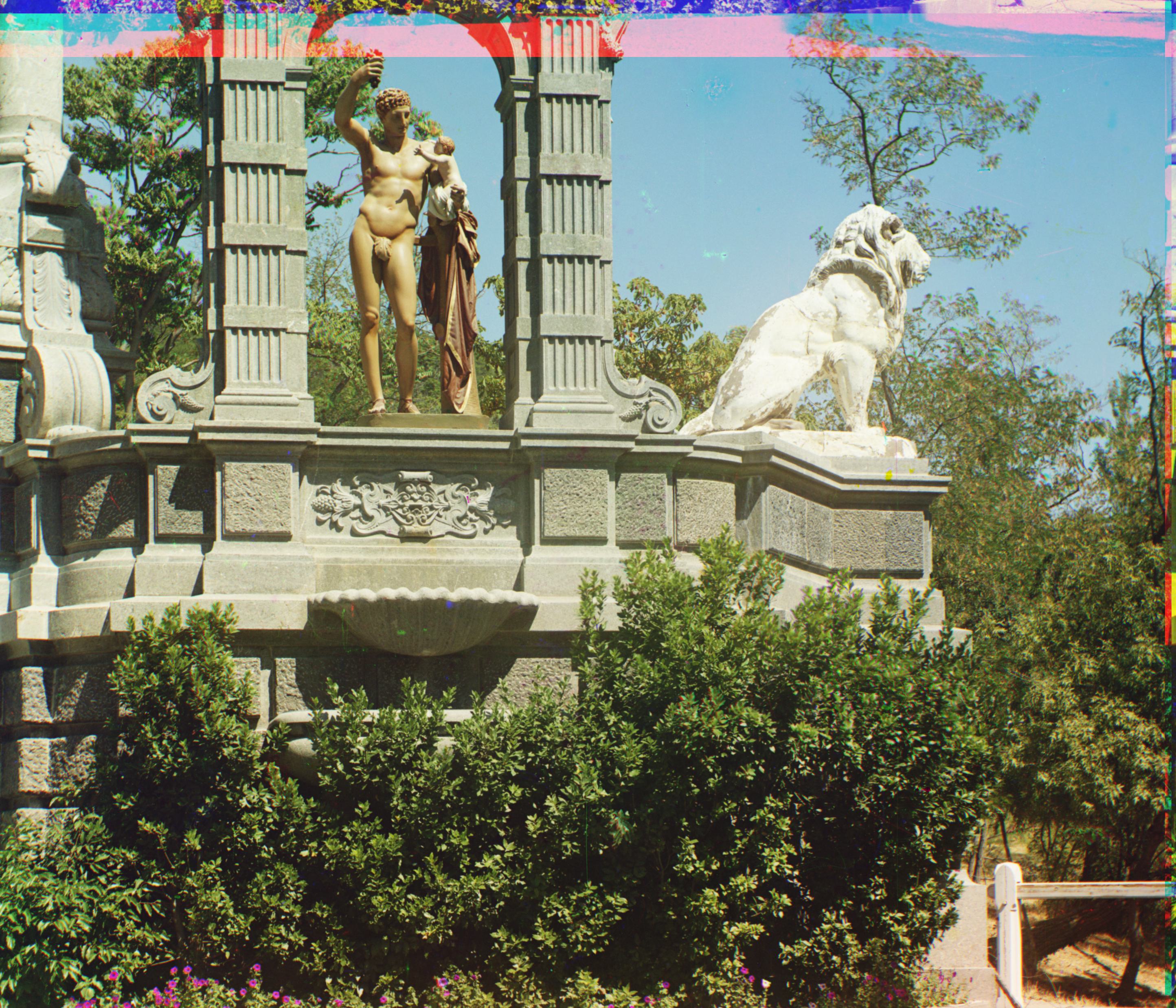
Sculpture
G: (33, -11)
R: (140, -27)

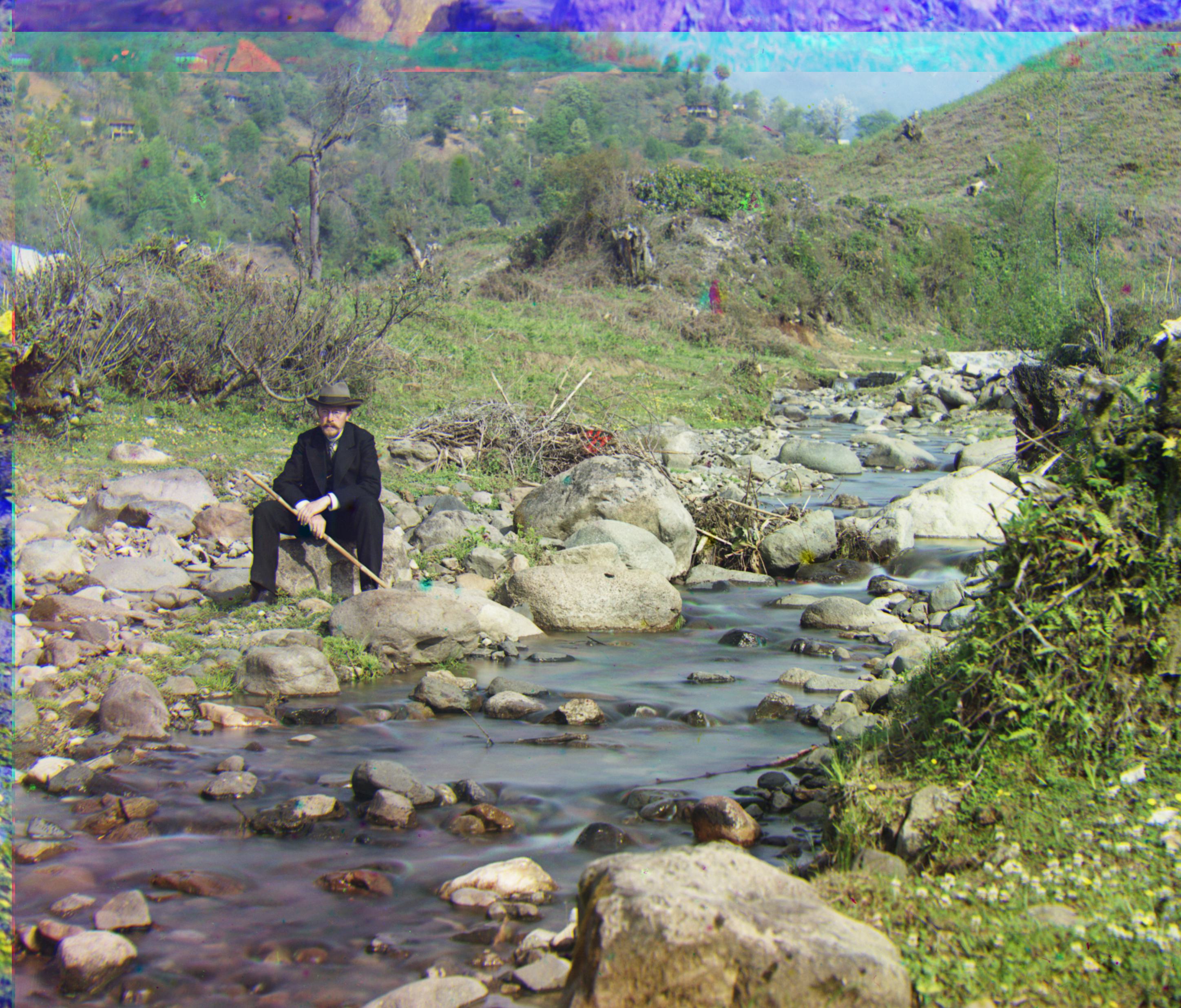
Self Portrait
G: (78, 29)
R: (176, 37)

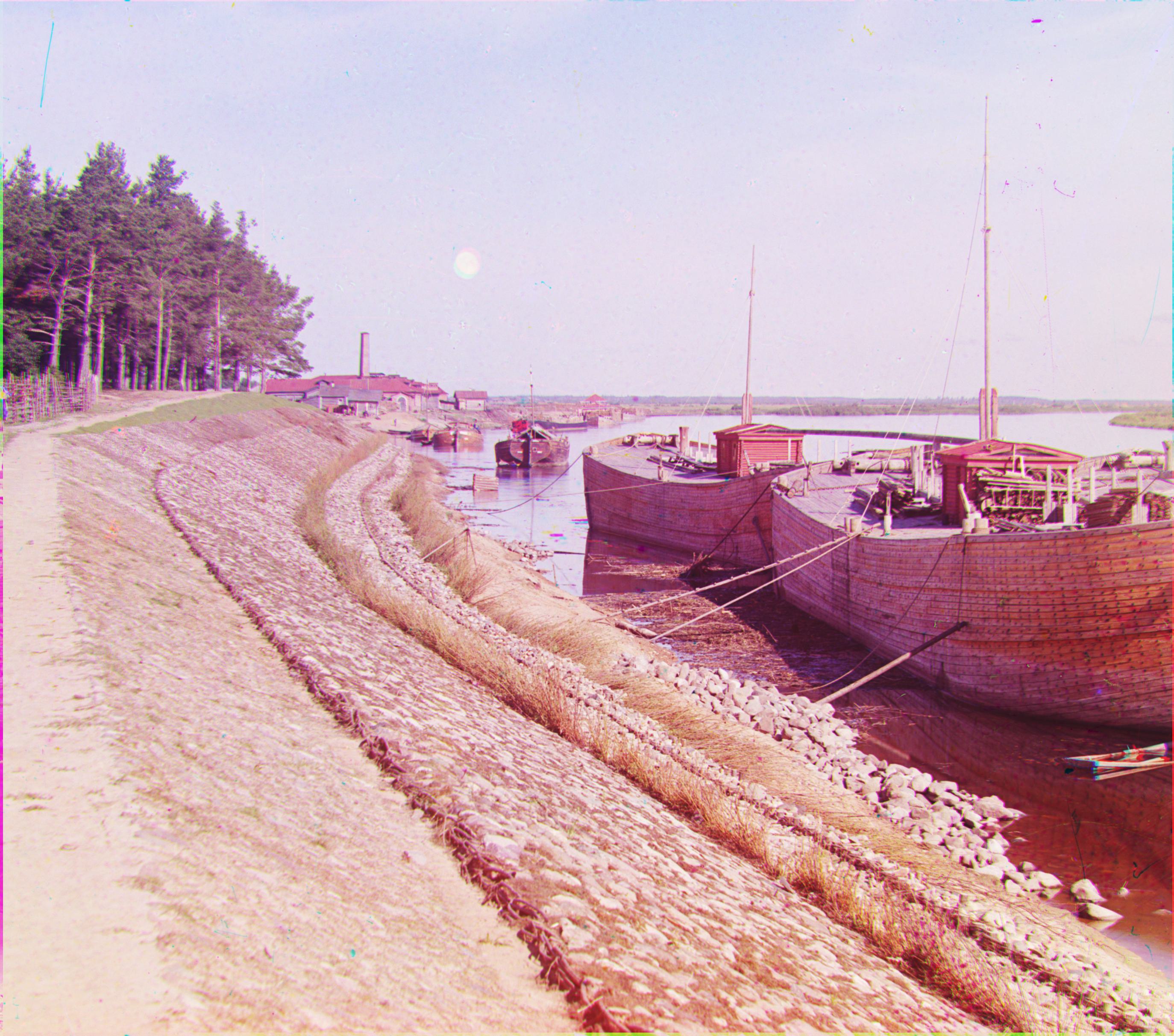
Vokhnovo
Self-chosen
G: (-8, 7)
R: (3, -4)

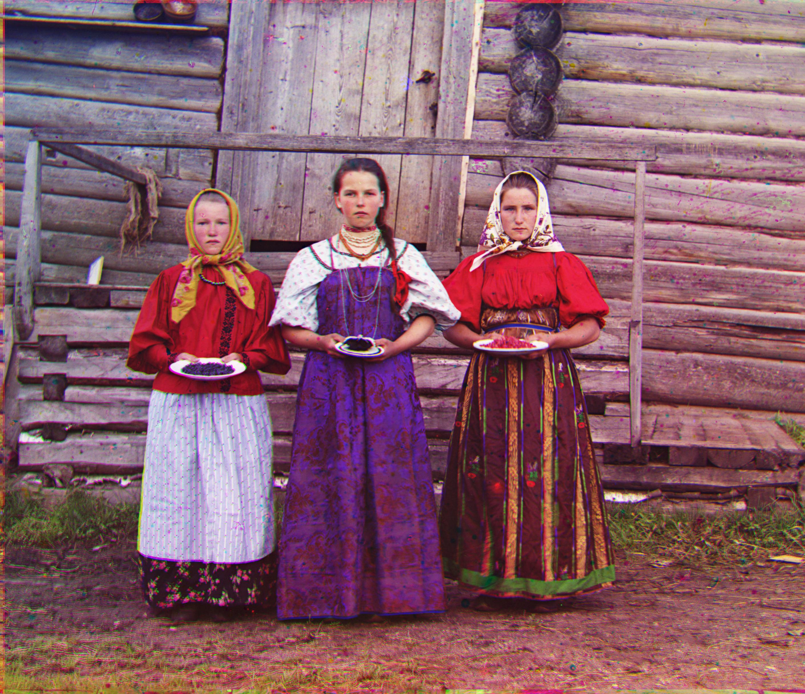
Three Girls
Self-chosen
G: (-16, 10)
R: (11, 17)

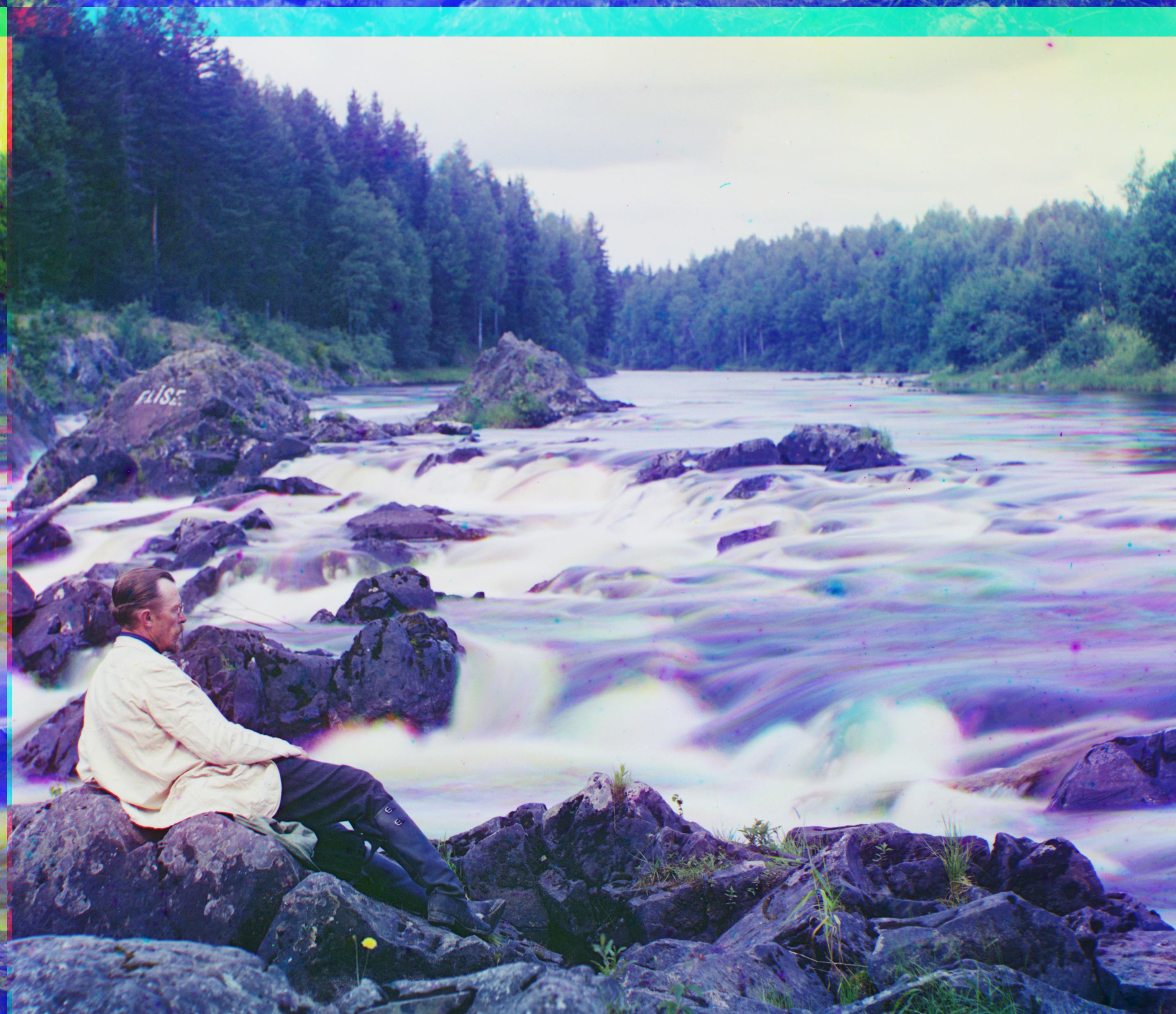
Kivach Waterfall
Self-chosen
G: (17, 17)
R: (89, 30)

* Emir image had alignment difficulties due to different brightness patterns across color channels

Implementation Details & Challenges

Normalization Strategy

I initially used simple division by 255 for normalization, but this led to graying of the output images (likely due to the initial pixel value ranges not spanning 0-255 but rather something like 50-100).

Min-max normalization was effective for handling the varying brightness ranges across different color channels and images, and resolved this graying issue.

The Emir Challenge

The Emir image was the image that aligned the worst compared to the others due to significantly different brightness patterns between color channels. The bright clothing in some channels appears dark in others, causing the NCC metric to fail.

Edge-based alignment methods (e.g. Sobel-filter or some other image-gradient process) that align based on the edges of the image would likely improve the alignment results.

Project 1: Images of the Russian Empire -- Colorizing the Prokudin-Gorksii Photo Collection